Semiconductor in Equilibrium

1 Introduction:

So far, we have considered a general crystal and attempted to determine certain properties of electrons in a single-crystal lattice by applying the concepts of quantum mechanics to this crystal. In this chapter, we will use the density of quantum states in the conduction band and valence band together with the Fermi–Dirac probability function to determine the electron concentration in the conduction band and the hole concentration in the valence band, respectively. We will also apply the concept of Fermi energy to semiconductor materials.

In this chapter, we consider a semiconductor in equilibrium. Equilibrium, or thermal equilibrium, means that there are no external influences acting on the semiconductor, such as an applied voltage, electric field, magnetic field, or temperature difference. Under these conditions, none of the properties of the semiconductor change with time; that is, they remain constant.

1.1 Charge Carriers in Semiconductors

Current, in the simplest terms, is the flow of charge; that is, when we talk about current, we are referring to moving charges. In a semiconductor, two types of charge carriers can contribute to the current: electrons and holes. We can regard holes as vacancies resulting from the absence of electrons, or directly as positively charged particles. Since the current in a semiconductor is largely determined by the number of electrons in the conduction band and the number of holes in the valence band, an important property of a semiconductor is the concentration of these charge carriers.

The concentrations of electrons and holes are related to two concepts we have discussed previously: the density of states function (DOS function) and the Fermi distribution function. We will first discuss these relationships conceptually; then, we will derive the concentrations of electrons and holes at thermal equilibrium in a more rigorous mathematical manner.

Distribution of Electrons and Holes at Equilibrium

The energy distribution of electrons in the conduction band can be determined by multiplying the density of allowed quantum states by the probability that a given state is occupied by an electron:

$$n(E) = g_c(E),f_F(E) \tag{1}$$

Here, $n(E)$ represents the electron concentration at energy $E$, $g_c(E)$ represents the density of states function in the conduction band, and $f_F(E)$ represents the Fermi–Dirac probability function. If we want to determine the total electron concentration in the conduction band, we integrate Equation (1) over all energies within the conduction band.

Similarly, the energy distribution of holes in the valence band is given by the product of the density of states in the valence band and the probability that a state is not occupied by an electron:

$$p(E) = g_v(E),[1 - f_F(E)] \tag{2}$$

Similarly, we can determine the total hole concentration by integrating Equation (2) over the entire valence band.

Here, we would like to make a brief reminder about the density of states (DoS), $g_c(E)$ and $g_v(E)$. The density of states is an energy-dependent function. Its unit is the number of states per unit volume per unit energy, $cm^{-3}eV^{-1}$. It tells us: "How many allowed quantum states are there per unit volume within a unit energy interval around the energy $E$?" In other words, it is a density function normalized with respect to both volume and energy. By itself, it does not give the number of electrons; it only tells us how many available states exist at a given energy.

The concentrations $n$ and $p$ (or $n(E)$ and $p(E)$) are, in fact, energy-dependent distribution functions. Their units are also $cm^{-3}eV^{-1}$, since they represent the number of available states multiplied by the probability that those states are occupied by electrons or holes, respectively.

However, when this distribution is integrated over energy (across the entire conduction or valence band), the energy unit cancels out, and the resulting $n$ or $p$ represents the actual carrier concentration, with units of $cm^{-3}$, i.e., the number of electrons or holes per unit volume. In short, while the density of states is a function distributed with respect to energy, the concentration is the energy-integrated form of this function, reduced to a single quantity.

To determine the electron and hole concentrations at thermal equilibrium, we need to know the position of the Fermi energy $E_F$ relative to the lower edge of the conduction band, $E_c$, and the upper edge of the valence band, $E_v$. For this purpose, let us first consider an intrinsic semiconductor. An ideal intrinsic semiconductor is a pure semiconductor that contains no dopant atoms or crystal defects (for example, pure silicon).

At $T = 0,\text{K}$, all states in the valence band of an intrinsic semiconductor are occupied by electrons, while all states in the conduction band are empty. Therefore, the Fermi energy must lie somewhere between $E_c$ and $E_v$ (the Fermi energy does not necessarily have to correspond to an allowed energy level).

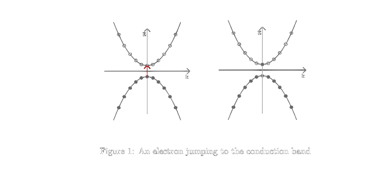
As the temperature begins to rise above $0,\text{K}$, electrons in the valence band gain thermal energy. Some electrons may acquire enough energy to transition into the conduction band. When an electron transitions from the valence band to the conduction band, an empty state, or a "hole," is created in the valence band (see Figure (1)). Thus, in an intrinsic semiconductor, electrons and holes are generated in pairs as a result of thermal energy; that is, the number of electrons in the conduction band is equal to the number of holes in the valence band. We will use this equality to derive the equations for the equilibrium charge-carrier concentrations.

1.2 $n_0 p_0$ Equations

If the effective masses of electrons and holes are not equal, the Fermi level shifts away from the midgap energy (the energy corresponding to the midpoint of the band gap) in order to maintain equal electron and hole concentrations.

Our primary goal was to determine the equilibrium charge-carrier concentrations. To carry out this derivation, we will need to introduce some new parameter definitions.

1.3 Electron Concentrations in Thermal Equilibrium

As stated previously, we can obtain the equation for the equilibrium concentration of electrons by integrating Equation (1) over all energies in the conduction band:

$$n_0 = \int g_c(E),f_F(E),dE \tag{3}$$

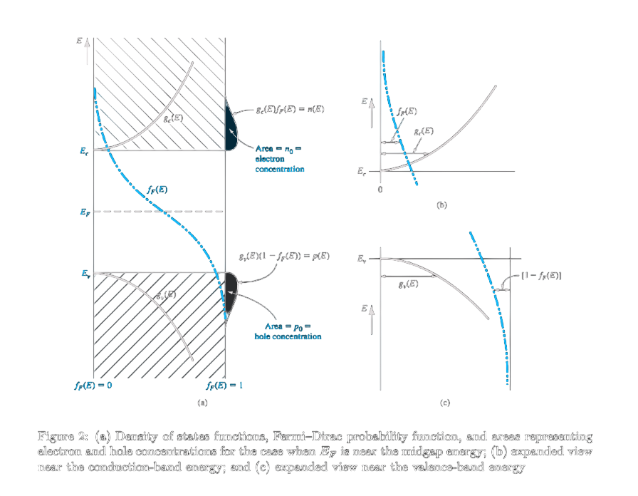
The lower limit of this integral is $E_c$, while the upper limit should correspond to the highest allowed energy in the conduction band. However, as shown in Figure 2a, since the Fermi probability function rapidly approaches zero as the energy increases, we can take the upper limit of the integral to be infinity.

We assume that the Fermi energy lies within the forbidden energy gap (band gap). For electrons in the conduction band,

$$E \geq E_c$$

If

$$E_c - E_F \gg kT,$$

then

$$E - E_F \gg kT.$$

Under these conditions, the Fermi probability function can be reduced to the Boltzmann approximation. Accordingly,

$$f_F(E) = \frac{1}{1 + \exp\left(\frac{E - E_F}{kT}\right)}$$

can be written as

$$f_F(E) \approx \exp\left(-\frac{E - E_F}{kT}\right). \tag{4}$$

The essential idea here is that when $E - E_F$ is much greater than $kT$, the 1 in the denominator of the Fermi–Dirac distribution can be neglected, and the function takes the form of the classical Boltzmann distribution.

Applying the Boltzmann approximation to Equation (3), the equilibrium electron concentration in the conduction band can be obtained from

$$n_0 = \int_{E_c}^{\infty} \frac{4\pi(2m_n^*)^{3/2}}{h^3},(E - E_c)^{1/2} \exp\left(-\frac{E - E_F}{kT}\right) dE. \tag{5}$$

The integral in Equation (5) can be solved more easily by making a change of variables. Let

$$\epsilon = \frac{E - E_c}{kT}.$$

Then, Equation (5) becomes

$$n_0 = \frac{4\pi(2m_n^* kT)^{3/2}}{h^3} \exp\left(-\frac{E_c - E_F}{kT}\right) \int_0^{\infty} \epsilon^{1/2} e^{-\epsilon}, d\epsilon. \tag{6}$$

This integral is a Gamma function, whose value is

$$\int_0^{\infty} \eta^{1/2} e^{-\eta}, d\eta = \frac{\sqrt{\pi}}{2}. \tag{7}$$

Thus, Equation (6) can be written as

$$n_0 = 2\left(\frac{2\pi m_n^* kT}{h^2}\right)^{3/2} \exp\left(-\frac{E_c - E_F}{kT}\right). \tag{8}$$

We can now define a parameter $N_c$:

$$N_c = 2\left(\frac{2\pi m_n^* kT}{h^2}\right)^{3/2}. \tag{9}$$

Here, $m_n^*$ is the density-of-states effective mass of the electron. Thus, the equilibrium electron concentration in the conduction band can be expressed as

$$n_0 = N_c \exp\left(-\frac{E_c - E_F}{kT}\right). \tag{10}$$

The parameter $N_c$ is called the effective density of states in the conduction band. If

$$m_n^* = m_0,$$

then, at $T = 300,\text{K}$, the effective density of states is approximately

$$N_c = 2.5 \times 10^{19}\ \text{cm}^{-3}.$$

This value is of the same order of magnitude as $N_c$ for most semiconductors.

When the effective mass of the electron is larger or smaller than $m_0$, the value of the effective density of states changes accordingly. Nevertheless, it remains of approximately the same order of magnitude. The most important result here is that as $E_F$ approaches $E_c$, the electron concentration in the conduction band increases exponentially.

1.4 Hole Concentrations in Thermal Equilibrium

Similarly, we can obtain the equation for the equilibrium hole concentration by integrating Equation (2) over all energies in the valence band:

$$p_0 = \int g_v(E),[1 - f_F(E)],dE. \tag{11}$$

The expression in square brackets can be written for states in the valence band ($E < E_v$) as

$$1 - f_F(E) = \frac{1}{1 + \exp\left(\frac{E_F - E}{kT}\right)}.$$

If

$$E_F - E_v \gg kT,$$

then

$$E_F - E \gg kT.$$

Under these conditions, the Fermi probability function reduces to a slightly different form of the Boltzmann approximation:

$$1 - f_F(E) \approx \exp\left(-\frac{E_F - E}{kT}\right). \tag{12}$$

Applying this approximation to Equation (11), the equilibrium hole concentration in the valence band can be written as

$$p_0 = \int_{-\infty}^{E_v} \frac{4\pi(2m_p^*)^{3/2}}{h^3},\sqrt{E_v - E}, \exp\left(-\frac{E_F - E}{kT}\right) dE. \tag{13}$$

As shown in Figure 2(a), the Fermi probability function for holes approaches zero as the energy decreases. Therefore, taking the lower limit of the integral in Equation (13) to be negative infinity does not affect the validity of the equation.

The integral in Equation (13) can likewise be simplified by making a change of variables. Let

$$\eta' = \frac{E_v - E}{kT}.$$

Then, Equation (13) becomes

$$p_0 = \frac{-4\pi(2m_p^* kT)^{3/2}}{h^3} \exp\left(-\frac{E_F - E_v}{kT}\right) \int_{+\infty}^{0} (\eta')^{1/2} \exp(-\eta'), d\eta'. \tag{14}$$

Note that the differential $dE$ is negative under this change of variables. Therefore, the order of the integration limits must be reversed. Using the Gamma function again, $p_0$ can be written as

$$p_0 = 2\left(\frac{2\pi m_p^* kT}{h^2}\right)^{3/2} \exp\left(-\frac{E_F - E_v}{kT}\right). \tag{15}$$

Here, $m_p^*$ is the density-of-states effective mass of the hole. We can define the parameter $N_v$, representing the effective density of states in the valence band, as

$$N_v = 2\left(\frac{2\pi m_p^* kT}{h^2}\right)^{3/2}. \tag{16}$$

Thus, the equilibrium hole concentration in the valence band can be expressed as

$$p_0 = N_v \exp\left(-\frac{E_F - E_v}{kT}\right). \tag{17}$$

For most semiconductors at $T = 300,\text{K}$, $N_v$ is also of the order of $10^{19},\text{cm}^{-3}$.

The effective density-of-states parameters $N_c$ and $N_v$ have fixed values for a given semiconductor material at a fixed temperature. Tables containing these values for different temperatures are commonly used.

1.5 Intrinsic Carrier Concentration

As mentioned previously, intrinsic semiconductors are pure semiconductors that contain no dopant atoms or crystal defects. Because of this property, the electron concentration in the conduction band is equal to the hole concentration in the valence band in an intrinsic semiconductor. Thus, the equality of the charge-carrier concentrations in an intrinsic semiconductor can be expressed as

$$n_i = p_i. \tag{18}$$

For simplicity, we will refer to $n_i$ as the intrinsic carrier concentration and use the notation $n_i$ instead of $p_i$ as well.

For intrinsic semiconductors, the Fermi energy level is denoted by $E_F = E_{Fi}$. Using Equations (10) and (17), we can write

$$n_0 = n_i = N_c \exp\left(-\frac{E_c - E_{Fi}}{kT}\right) \tag{19}$$

and

$$p_0 = p_i = n_i = N_v \exp\left(-\frac{E_{Fi} - E_v}{kT}\right). \tag{20}$$

Multiplying Equations (19) and (20), we obtain

$$n_i^2 = N_c N_v \exp\left(-\frac{E_c - E_v}{kT}\right) = N_c N_v \exp\left(-\frac{E_g}{kT}\right). \tag{21}$$

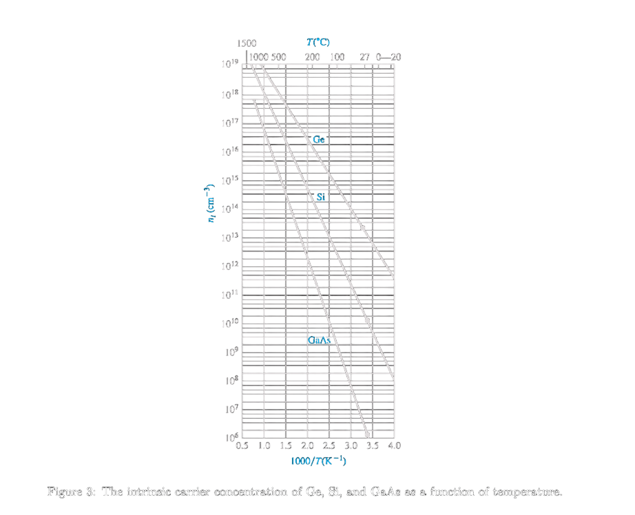
Here, $E_g$ is the band-gap energy. The most important conclusion that can be drawn from Equation (21) is that, for a given semiconductor at a fixed temperature, the intrinsic carrier concentration $n_i$ is a constant independent of the Fermi energy. In addition, the equation shows that the carrier concentration is highly dependent on temperature. This temperature dependence is shown for Ge, Si, and GaAs in Figure 3.

1.6 The Intrinsic Fermi-Level Position

The position of the Fermi level is closely related to the effective masses of the charge carriers. Let us now examine this relationship for intrinsic semiconductors.

We have seen that, in an intrinsic semiconductor, the electron concentration must be equal to the hole concentration. Therefore, we can set Equations (19) and (20) equal to each other:

$$N_c \exp\left(-\frac{E_c - E_{Fi}}{kT}\right) = N_v \exp\left(-\frac{E_{Fi} - E_v}{kT}\right). \tag{22}$$

Taking the natural logarithm of both sides of Equation (22) and solving for $E_{Fi}$, we obtain

$$E_{Fi} = \frac{1}{2}(E_c + E_v) + \frac{1}{2}kT \ln\left(\frac{N_v}{N_c}\right). \tag{23}$$

Finally, we can use the expressions for $N_c$ and $N_v$ defined in Equations (9) and (16), respectively. We can also rewrite the midgap energy, by definition, as

$$\frac{1}{2}(E_c + E_v) = E_{midgap}.$$

Thus,

$$E_{Fi} = E_{midgap} + \frac{3}{4}kT \ln\left(\frac{m_p^*}{m_n^*}\right), \tag{24}$$

or equivalently,

$$E_{Fi} - E_{midgap} = \frac{3}{4}kT \ln\left(\frac{m_p^*}{m_n^*}\right). \tag{25}$$

The main conclusions we should draw from Equation (24) are:

• The Fermi level shifts above the center of the band gap when $m_p^* > m_n^*$, and below the center when $m_p^* < m_n^*$. In other words, the Fermi level shifts away from the band with the higher density of states in order to maintain the balance between the available states. This occurs because the number of electrons and holes must remain equal in an intrinsic semiconductor.
• When the effective masses of the charge carriers are equal, the Fermi level lies exactly at the center of the band gap.

In this article, we have learned how to determine the charge-carrier concentrations of intrinsic semiconductors at equilibrium. We have also examined the relationship between the Fermi energy level and the effective-mass parameter. In the next article, we will deepen our understanding by considering extrinsic semiconductors, which are widely used in semiconductor technology.

References

• Semiconductor Physics And Devices by Donald A. Neamen Third Edition
• The Oxford Solid State Basics by Steven H. Simon
• https://www.doitpoms.ac.uk/tlplib/semiconductors/index.php