The Schrödinger Equation

In classical mechanics, a particle’s state can be specified exactly at any instant using physical quantities such as position and momentum. Experiments at atomic and subatomic scales, however, have shown this description to be inadequate.

At these scales, particles do not follow definite classical trajectories. Instead, a particle’s state is represented by a complex-valued function called the wave function.

The wave function

$$\psi(r,t)$$

is defined as above and contains the particle’s state at position $r$ in space and time $t$.

The wave function itself is not directly observable. Physical meaning is associated with its absolute square, which gives the probability of finding the particle in a particular region of space.

The probability density is therefore

$$\rho(r,t) = |\psi(r,t)|^2$$

defined as shown.

For a wave function to be physically meaningful, it must be normalized:

$$\int |\psi(r,t)|^2 \, d\tau = 1$$

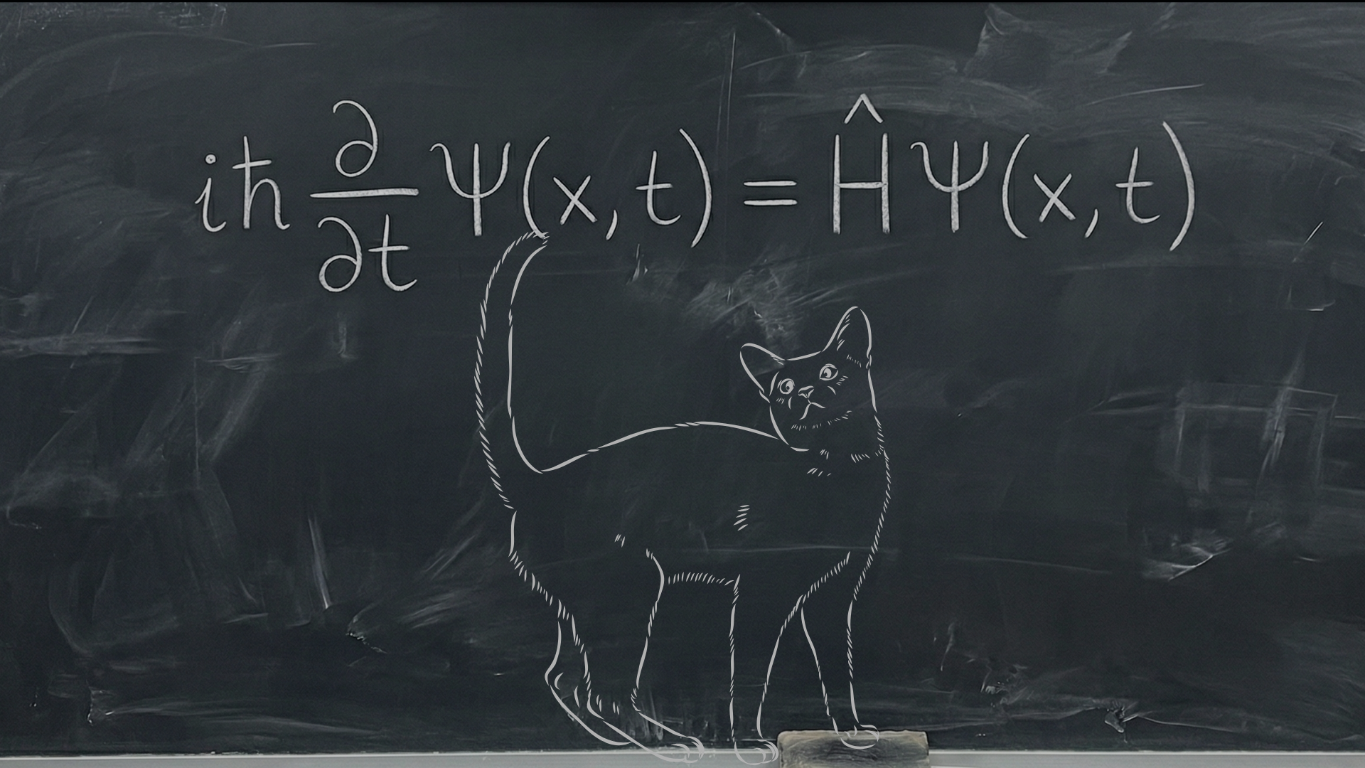
The fundamental problem of quantum mechanics is to determine how the wave function evolves in time. The governing equation is the Schrödinger equation.

Wave–Particle Duality and the de Broglie Hypothesis

Classical physics treats waves and particles as entirely distinct. Waves propagate through space and exhibit interference and diffraction, while particles are viewed as pointlike entities with definite positions and trajectories.

Experiments in the early twentieth century showed that this distinction fails microscopically. In particular, the photoelectric effect and Compton scattering revealed that light exhibits both wave and particle properties.
From these results, Louis de Broglie proposed that the wave–particle duality of light should apply to every material particle. This is a fundamental assumption of quantum mechanics.

Under the de Broglie hypothesis, a particle of momentum $p$ can be assigned a wavelength. Using Planck’s constant, it is

$$\lambda = \frac{h}{p}$$

expressed as above.

Particles with large momentum thus have very short wavelengths, making wave effects negligible and their behavior classical. Wave properties become pronounced for particles with small momentum.

A de Broglie wave is not a physical wave propagating through space in the classical sense. It forms the mathematical basis of the wave function describing the particle’s quantum state and is therefore crucial to the transition to the wave-function concept.

Wave character can be represented by a plane-wave solution:

$$\psi(r,t) = A e^{i(\mathbf{k}\cdot\mathbf{r}-\omega t)}$$

Here, $\mathbf{k}$ is the wave vector and $\omega$ the angular frequency. These quantities are connected to energy and momentum through

$$\mathbf{p} = \hbar \mathbf{k}, \qquad E = \hbar \omega$$

the relations above.

These expressions show how energy and momentum are related to wave properties in quantum mechanics and underpin the operator formalism.

Operators and Physical Quantities

In classical mechanics, position, momentum, and energy are measurable physical quantities. In quantum mechanics, they are represented not directly by numbers but by operators.

An operator acts on a wave function to specify measurement outcomes for the corresponding physical quantity. This approach forms the mathematical foundation of quantum mechanics.

Momentum Operator

The plane-wave solution

$$\psi(r,t) = A e^{i(\mathbf{k}\cdot\mathbf{r}-\omega t)}$$

can be used to examine momentum.

Taking the spatial derivative of the plane wave gives

$$\nabla \psi = i\mathbf{k}\psi$$

the result above. Combining it with the relation between momentum and wave vector,

$$\mathbf{p} = \hbar \mathbf{k}$$

reveals the quantum-mechanical operator corresponding to momentum.

The momentum operator is therefore

$$\hat{\mathbf{p}} = -i\hbar \nabla$$

defined as shown.

Acting on a wave function, it yields possible momentum measurement results.

Energy Operator

The same approach applies to energy. Differentiating the plane-wave solution with respect to time gives

$$\frac{\partial \psi}{\partial t} = -i\omega \psi$$

the result above.

Using the relation between energy and angular frequency,

$$E = \hbar \omega$$

the energy operator is

$$\hat{E} = i\hbar \frac{\partial}{\partial t}$$

defined as shown.

This operator determines the wave function’s time dependence and underlies energy measurements.

These operator definitions will be used directly in constructing the Schrödinger equation.

The Time-Dependent Schrödinger Equation

A central aim of quantum mechanics is to determine how a particle’s wave function evolves in time. The equation describing this evolution is the time-dependent Schrödinger equation.

In classical mechanics, a particle’s total energy is the sum of its kinetic and potential energies:

$$E = \frac{p^2}{2m} + V(r,t)$$

In quantum mechanics, this expression is not used directly; energy and momentum are replaced by their respective operators. Thus, the substitution

$$E \longrightarrow \hat{E}, \qquad \mathbf{p} \longrightarrow \hat{\mathbf{p}}$$

is made.

Substituting the energy and momentum operators gives

$$\hat{E}\psi = \left( \frac{\hat{p}^{2}}{2m} + V(r,t) \right)\psi$$

the expression above.

The square of the momentum operator is

$$\hat{p}^{2} = (-i\hbar\nabla)^2 = -\hbar^2 \nabla^2$$

as shown.

Writing the energy and momentum operators explicitly, the time-dependent Schrödinger equation

$$i\hbar \frac{\partial \psi(r,t)}{\partial t} = \left[ -\frac{\hbar^2}{2m}\nabla^2 + V(r,t) \right]\psi(r,t)$$

takes this form.

This is the fundamental differential equation governing a particle’s dynamics in quantum mechanics.

The Time-Independent Schrödinger Equation

In many physical problems, the potential energy has no explicit time dependence. The potential can then be written

$$V(r,t) = V(r)$$

as above.

A time-independent potential allows the wave function to be separated into spatial and temporal factors, a method called separation of variables.

Let the wave function be written

$$\psi(r,t) = \phi(r)\, T(t)$$

in this form.

Substitution into the time-dependent Schrödinger equation produces two separate equations because the space and time variables are independent.

For the temporal part,

$$i\hbar \frac{1}{T}\frac{dT}{dt} = E$$

is obtained, with solution

$$T(t) = e^{-iEt/\hbar}$$

as shown.

For the spatial part, one obtains

$$-\frac{\hbar^2}{2m}\nabla^2 \phi(r) + V(r)\phi(r) = E\phi(r)$$

the equation above.
This is called the time-independent Schrödinger equation.

Besides being a differential equation, it is an eigenvalue problem. The energy $E$ represents its eigenvalues, while $\phi(r)$ represents its eigenfunctions.

Quantum-mechanical energy levels are therefore generally discrete, and the system’s physical properties are determined by these eigenvalues.

Stationary States and the Probability Interpretation

Solutions of the time-independent Schrödinger equation are called the system’s stationary states. Their time dependence consists solely of a phase factor.

For stationary states, the wave function is written

$$\psi(r,t) = \phi(r)e^{-iEt/\hbar}$$

as shown.

Taking the absolute square of this wave function gives

$$|\psi(r,t)|^2 = |\phi(r)|^2$$

the result above. As seen, the probability density is time-independent.

Thus, in a stationary state, the particle’s spatial probability distribution does not change with time. This property defines the concept of a stationary state.

Normalization

A physically meaningful wave function must be normalized. This means the total probability of finding the particle somewhere in space equals one:

$$\int |\psi(r,t)|^2 \, d\tau = 1$$

For stationary states, this expression

$$\int |\phi(r)|^2 \, d\tau = 1$$

simplifies as shown.

This integral fixes the wave-function amplitude and gives physical meaning to constants arising in the solution.

Physical Interpretation

Stationary states have precisely defined energies. Energy measurements in such a state always yield the same result.

Other physical quantities, such as position, are not definite and are described only by probability distributions. This is one of quantum mechanics’ most fundamental departures from classical mechanics.

The Schrödinger Equation in Spherical Coordinates

In a centrally symmetric system, the potential energy depends only on the particle’s distance from the origin. Such potentials

$$V(r) = V(r)$$

are written as above, and spherical coordinates greatly simplify the problem.

Spherical coordinates are defined by $r$, $\theta$, and $\varphi$. In these coordinates, the Laplacian

$$\nabla^2 = \frac{1}{r^2}\frac{\partial}{\partial r}\left(r^2 \frac{\partial}{\partial r}\right) + \frac{1}{r^2 \sin\theta}\frac{\partial}{\partial \theta}\left(\sin\theta \frac{\partial}{\partial \theta}\right) + \frac{1}{r^2 \sin^2\theta}\frac{\partial^2}{\partial \varphi^2}$$

is written in the form above.

Substituting this expression into the time-independent Schrödinger equation gives

$$-\frac{\hbar^2}{2m}\nabla^2 \psi(r,\theta,\varphi) + V(r)\psi(r,\theta,\varphi) = E\psi(r,\theta,\varphi)$$

the equation above.

For central potentials, the wave function can be separated:

$$\psi(r,\theta,\varphi) = R(r)\, Y(\theta,\varphi)$$

Substitution into the Schrödinger equation separates the radial and angular parts.

Angular Equation

The angular part depends only on $\theta$ and $\varphi$ and can be written

$$\hat{L}^2 Y(\theta,\varphi) = \ell(\ell+1)\hbar^2 Y(\theta,\varphi)$$

Here, $\hat{L}^2$ is the squared angular-momentum operator. The quantum number $\ell$ determines the magnitude of angular momentum.

The solutions are called spherical harmonics and are denoted

$$Y_{\ell}^{m}(\theta,\varphi)$$

as shown.

Radial Equation

The radial equation is

$$-\frac{\hbar^2}{2m} \left[ \frac{1}{r^2}\frac{d}{dr}\left(r^2 \frac{dR}{dr}\right) - \frac{\ell(\ell+1)}{r^2}R \right] + V(r)R = ER$$

as shown.

This equation is fundamental to solving central-potential problems, particularly systems such as the hydrogen atom.

Operators in Quantum Mechanics

Unlike classical mechanics, quantum mechanics represents physical quantities not directly by numbers but by operators. Acting on a wave function, these operators reveal information corresponding to measurable quantities.

Every measurable physical quantity has an associated operator. These are generally linear differential operators and form the mathematical foundation of quantum mechanics.

Linearity

An operator $\hat{A}$ satisfies linearity on wave functions. This property is

$$\hat{A}(a\psi_1 + b\psi_2) = a\hat{A}\psi_1 + b\hat{A}\psi_2$$

expressed as above, where $a$ and $b$ are constant coefficients.

Linearity is the mathematical foundation of the superposition principle in quantum mechanics.

Basic Operators

Some of the most frequently used operators in quantum mechanics are:

• Position operator:

$$\hat{\mathbf{r}} = \mathbf{r}$$

• Momentum operator:

$$\hat{\mathbf{p}} = -i\hbar\nabla$$

• Energy (Hamiltonian) operator:

$$\hat{H} = -\frac{\hbar^2}{2m}\nabla^2 + V(r,t)$$

These operators are the fundamental building blocks of the Schrödinger equation.

Eigenvalue Problem

An operator eigenvalue problem is defined by

$$\hat{A}\psi = a\psi$$

the expression above, where $a$ is the operator’s eigenvalue.

A quantum measurement must yield one of the corresponding operator’s eigenvalues. The generally discrete nature of measurement outcomes therefore arises from the operators’ eigenvalue structure.

Hermitian Operators

The eigenvalues of operators corresponding to physically measurable quantities must be real. Operators satisfying this condition are called Hermitian operators.

For an operator to be Hermitian, it must satisfy

$$\int \psi_1^*(\hat{A}\psi_2)\, d\tau = \int (\hat{A}\psi_1)^* \psi_2 \, d\tau$$

the condition above.

This guarantees that measurements of physical quantities such as energy, momentum, and position yield real values.

Some Physical Operators

Every measurable physical quantity in quantum mechanics has a corresponding operator. This section presents the most frequently used basic physical operators and their mathematical expressions.

Momentum Operators

The components of the momentum operator in three-dimensional space are defined as

$$\hat{P}_x = -i\hbar \frac{\partial}{\partial x}, \qquad \hat{P}_y = -i\hbar \frac{\partial}{\partial y}, \qquad \hat{P}_z = -i\hbar \frac{\partial}{\partial z}$$

The vector form of the momentum operator is

$$\hat{\mathbf{P}} = -i\hbar\nabla$$

as shown.

These operators describe a particle’s translational motion through space.

Energy Operator

The operator corresponding to energy contains a time derivative and is

$$\hat{E} = i\hbar \frac{\partial}{\partial t}$$

the expression above.

The Hamiltonian operator represents the system’s total energy and is defined

$$\hat{H} = -\frac{\hbar^2}{2m}\nabla^2 + V(r,t)$$

as shown.

Through the time-dependent Schrödinger equation, the Hamiltonian’s eigenvalues correspond to energy in energy-eigenvalue problems.

The Hamiltonian represents the system’s total energy.

Angular-Momentum Operators

The angular-momentum operator is defined by the vector product of the position and momentum operators:

$$\hat{\mathbf{L}} = \hat{\mathbf{r}} \times \hat{\mathbf{P}}$$

Writing its components explicitly gives

$$\hat{L}_x = -i\hbar \left( y\frac{\partial}{\partial z} - z\frac{\partial}{\partial y} \right)$$ $$\hat{L}_y = -i\hbar \left( z\frac{\partial}{\partial x} - x\frac{\partial}{\partial z} \right)$$ $$\hat{L}_z = -i\hbar \left( x\frac{\partial}{\partial y} - y\frac{\partial}{\partial x} \right)$$

The square of angular momentum is defined

$$\hat{L}^2 = \hat{L}_x^2 + \hat{L}_y^2 + \hat{L}_z^2$$

as shown.

These operators are fundamental to central-potential problems and are directly related to the Schrödinger equation in spherical coordinates.

Commutation Relations

The fundamental commutation relation between momentum and position is

$$[\hat{x},\hat{P}_x] = i\hbar$$

For angular-momentum operators,

$$[\hat{L}_x,\hat{L}_y] = i\hbar \hat{L}_z$$

and cyclic permutations hold.

These commutation relations determine whether observables can be measured simultaneously with certainty and form the mathematical basis of the uncertainty principle.

The Uncertainty Principle

In quantum mechanics, not all of a particle’s physical quantities can be measured simultaneously with arbitrary precision. This fundamental limitation is the Heisenberg uncertainty principle.

It arises not from shortcomings in measuring instruments but directly from the mathematical structure of quantum mechanics.

Position–Momentum Uncertainty

The fundamental commutation relation between the position and momentum operators is

$$[\hat{x},\hat{P}_x] = i\hbar$$

as shown.

This relation connects the uncertainties in position and momentum:

$$\Delta x\, \Delta P_x \geq \frac{\hbar}{2}$$

Here, $\Delta x$ and $\Delta P_x$ are the standard deviations of position and momentum, respectively.

The more precisely a particle’s position is known, the more uncertain its momentum becomes.

Energy–Time Uncertainty

Energy and time obey a similar uncertainty relation:

$$\Delta E\, \Delta t \geq \frac{\hbar}{2}$$

Energy–time uncertainty differs from position–momentum uncertainty. Time is not defined as an operator in quantum mechanics, so this uncertainty arises not directly from a commutation relation but from the system’s temporal evolution.

Angular-Momentum Uncertainty

The angular-momentum components satisfy the commutation relations

$$[\hat{L}_x,\hat{L}_y] = i\hbar \hat{L}_z$$

Consequently, all angular-momentum components cannot be measured simultaneously with certainty. However, $\hat{L}^2$ and $\hat{L}_z$ can have definite values simultaneously.

This is the fundamental reason angular-momentum quantum numbers arise.

Physical Interpretation

The uncertainty principle shows that particles cannot be described by classical trajectories. Their behavior in quantum mechanics is probabilistic.

This follows directly from the spatial extent of the wave function and is one of quantum mechanics’ most fundamental conceptual consequences.