The Higgs Mechanism

The Higgs Mechanism: What Actually Happens When a Field “Gives Mass”?

The Higgs mechanism is often summarized in a single sentence: “Particles acquire mass by interacting with the Higgs field.” The sentence is not entirely wrong, but it conceals almost all the mechanism’s real beauty. The problem we are trying to solve is not that an invisible medium in empty space slows particles down. Even the phrase “acquire mass” is slightly dangerous: it sounds as though a physically massless $W$ boson exists first and then picks up mass while passing through the Higgs field. What we actually do is redefine the physical excitations around the vacuum of the theory using the correct variables.

In this article, we will first establish where the problem comes from. We will then explicitly derive the spontaneous breaking of a global symmetry, the Mexican-hat potential, and Goldstone’s theorem. Next, we will couple the same system to a local $U(1)$ symmetry and work through the Abelian Higgs mechanism step by step. Finally, we will carry the calculation into the real world, namely the electroweak example

$$SU(2)_L\times U(1)_Y\longrightarrow U(1)_{\mathrm{em}}$$

Together we will derive the masses of the $W^\pm$ and $Z$, why the photon remains massless, how fermions obtain mass terms through Yukawa interactions, and why only one physical scalar remains.

1. Why does a mass term cause trouble?

For a free, real scalar field, there is no problem with writing

$$\mathcal L_{\mathrm{scalar}} =\frac12\partial_\mu\phi\,\partial^\mu\phi-\frac12m^2\phi^2$$

Likewise, for a free Dirac field,

$$\mathcal L_{\mathrm{Dirac}} =\bar\psi(i\gamma^\mu\partial_\mu-m)\psi$$

is a valid Lorentz scalar. At first glance, we might also want to add a mass directly to a vector field:

$$\mathcal L_{\mathrm{Proca}} =-\frac14F_{\mu\nu}F^{\mu\nu} +\frac12m_A^2A_\mu A^\mu .$$

This is Proca theory, which describes a free massive spin-1 field. Lorentz symmetry is not the problem. The problem arises when $A_\mu$ is a gauge field. Under an Abelian gauge transformation,

$$A_\mu(x)\longrightarrow A_\mu(x)+\partial_\mu\alpha(x)$$

the field strength $F_{\mu\nu}=\partial_\mu A_\nu-\partial_\nu A_\mu$ is unchanged, whereas

$$A_\mu A^\mu \longrightarrow A_\mu A^\mu +2A^\mu\partial_\mu\alpha +\partial_\mu\alpha\,\partial^\mu\alpha$$

Thus a bare $m_A^2A_\mu A^\mu/2$ term is not gauge invariant.

Saying “then let us abandon gauge invariance” does not work, especially in non-Abelian theories. Gauge structure is not merely an aesthetic symmetry; it organizes the form of the interactions, the Ward–Takahashi or Slavnov–Taylor identities, the cancellation of unphysical polarizations from amplitudes, and the high-energy consistency of the theory. Adding Proca masses to the $W$ and $Z$ by hand makes scattering amplitudes of longitudinal polarizations grow uncontrollably with energy. A few sections from now, we will calculate how this growth threatens perturbative unitarity at a scale of roughly $1\ \mathrm{TeV}$.

There is a separate problem on the fermion side of the electroweak theory. The left-handed electron $e_L$ is one component of a weak-isospin doublet:

$$L_L= \begin{pmatrix} \nu_{eL}\\ e_L \end{pmatrix},$$

whereas the right-handed electron $e_R$ is an $SU(2)_L$ singlet. The Dirac mass

$$-m_e\bar e e =-m_e(\bar e_L e_R+\bar e_R e_L)$$

directly connects the left- and right-handed fields. Because these two fields transform differently under $SU(2)_L\times U(1)_Y$, however, the term is not electroweak gauge invariant.

The mechanism we seek must accomplish three things at once:

1. It must preserve the gauge-invariant structure of the Lagrangian density.
2. It must produce massive $W^\pm$, $Z$, and fermions in the physical spectrum around the vacuum.
3. It must preserve the cancellations that make the theory consistent at high energy.

This is precisely where the Higgs mechanism succeeds. Rather than attaching mass terms from the outside, we write gauge-invariant interactions and treat masses as the quadratic parts of those interactions expanded around the chosen vacuum.

2. Spontaneous symmetry breaking

Let us begin with a real scalar field:

$$\mathcal L =\frac12(\partial_\mu\phi)^2-V(\phi), \qquad V(\phi)=\frac12\mu^2\phi^2+\frac{\lambda}{4}\phi^4, \qquad \lambda>0.$$

The potential is invariant under $\phi\mapsto-\phi$; there is a $\mathbb Z_2$ symmetry. To find the vacua, we look for the minima of the potential among constant field configurations:

$$\frac{dV}{d\phi} =\phi(\mu^2+\lambda\phi^2)=0.$$

This gives two cases:

• If $\mu^2>0$, the only minimum is at $\phi=0$.
• If $\mu^2<0$, then $\phi=0$ is a maximum and there are two minima.

In the second case, writing $\mu^2=-m^2$ with $m^2>0$ gives

$$V(\phi) =-\frac12m^2\phi^2+\frac{\lambda}{4}\phi^4, \qquad \phi_{\mathrm{vac}}=\pm v, \qquad v^2=\frac{m^2}{\lambda}.$$

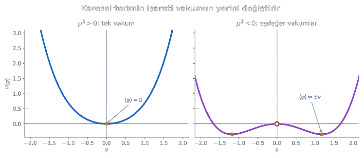
The Lagrangian density is still symmetric under $\phi\mapsto-\phi$. But once we choose one of the vacua, say $+v$, that vacuum does not map to itself under the transformation; it maps to $-v$. This is where the word “spontaneous” comes from: we have not added a symmetry-breaking term to the equations, but the ground state about which we perturb breaks the symmetry.

Around the chosen vacuum, write

$$\phi(x)=v+h(x)$$

Substituting into the potential and using $v^2=m^2/\lambda$, we obtain

$$V(v+h) =V(v)+m^2h^2+\lambda vh^3+\frac{\lambda}{4}h^4.$$

Because the standard mass term in the Lagrangian density is $-\frac12m_h^2h^2$,

$$m_h^2=2m^2=2\lambda v^2$$

The important point is this:

A field’s mass is the curvature of the potential at the chosen vacuum. For one field, $m_h^2=V''(v)$; for several fields, the mass-squared matrix is the Hessian of the potential.

The symmetry in this example is not continuous. There is no direction corresponding to continuous motion between the two vacua. Consequently, there is no Goldstone mode of the kind we will encounter shortly.

2.1 Complex field and the Mexican hat

Now consider a single complex scalar field:

$$\phi(x)=\frac{1}{\sqrt{2}}\bigl(\phi_1(x)+i\phi_2(x)\bigr),$$

with

$$\mathcal L =\partial_\mu\phi^\ast\partial^\mu\phi -V(\phi), \qquad V(\phi)=-\mu^2|\phi|^2+\lambda|\phi|^4, \qquad \mu^2,\lambda>0$$

The theory is invariant under the global transformation

$$\phi(x)\longrightarrow e^{i\alpha}\phi(x), \qquad \alpha=\text{sabit}$$

The word “global” matters: the same $\alpha$ is used at every point in spacetime.

The minimum condition is

$$\frac{\partial V}{\partial |\phi|} =-2\mu^2|\phi|+4\lambda|\phi|^3=0$$

The symmetry-breaking minima lie on the circle

$$|\phi|^2=\frac{\mu^2}{2\lambda}\equiv\frac{v^2}{2}, \qquad v^2=\frac{\mu^2}{\lambda}$$

In terms of the real components,

$$V(\phi_1,\phi_2) =\frac{\lambda}{4} \left(\phi_1^2+\phi_2^2-v^2\right)^2 -\frac{\lambda v^4}{4}$$

The final constant does not affect the classical field equations; it only fixes the zero of the potential. In Figure 2, the W-shaped curve on the left is a cross-section along the $\phi_2=0$ direction in field space. The minima $\varphi=\pm v$ in this cross-section are the two points where the section intersects the single vacuum circle shown on the right in the two-dimensional field space.

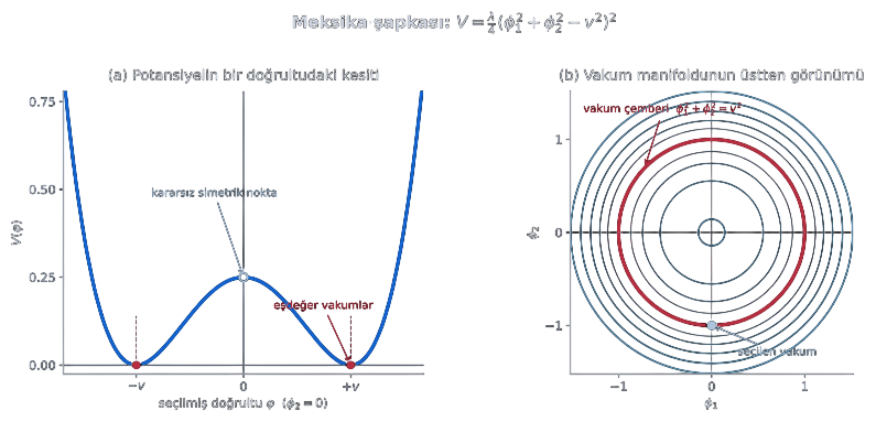
Every point along the brim of the hat has the same energy. We call this set of minima the vacuum manifold:

$$\mathcal M_{\mathrm{vac}}\simeq S^1.$$

Choose a vacuum:

$$\langle\phi\rangle=\frac{v}{\sqrt{2}}.$$

This choice is arbitrary; a choice with any other phase can be carried into this one by a global $U(1)$ transformation. Once we have made the choice and described small oscillations around it, however, we see two distinct kinds of motion: perpendicular radial motion and angular motion.

###Cartesian parametrization

Let

$$\phi(x)=\frac{1}{\sqrt{2}}\bigl[v+h(x)+i\pi(x)\bigr]$$

Expanding the potential to quadratic order gives

$$V =V_0+\frac12(2\lambda v^2)h^2 +0\times\frac12\pi^2+\mathcal O(\text{alan}^3)$$

Therefore,

$$m_h^2=2\lambda v^2=2\mu^2, \qquad m_\pi^2=0.$$

As $h$ moves radially, it feels the slope of the potential. The field $\pi$ lies tangent to the circle of minima; because the potential does not vary in that direction, it is massless.

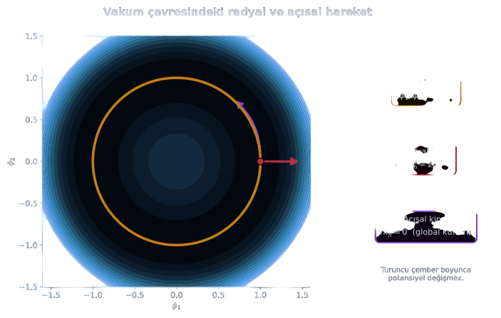
The same geometry is even more transparent in polar variables:

$$\phi(x) =\frac{v+h(x)}{\sqrt{2}} \exp\left(\frac{i\pi(x)}{v}\right).$$

The kinetic term becomes

$$\partial_\mu\phi^\ast\partial^\mu\phi =\frac12(\partial_\mu h)^2 +\frac12\left(1+\frac{h}{v}\right)^2(\partial_\mu\pi)^2$$

while the potential depends only on $h$:

$$V =\frac{\lambda}{4}\left[(v+h)^2-v^2\right]^2 -\frac{\lambda v^4}{4}.$$

There is no non-derivative $\pi$ term for the field $\pi^2$. When an exact global continuous symmetry is spontaneously broken, the existence of the massless mode is protected by Goldstone’s theorem.

3. What does Goldstone’s theorem tell us?

Let $J^\mu$ be the Noether current of a global continuous symmetry:

$$\partial_\mu J^\mu=0, \qquad Q=\int d^3x\,J^0(x).$$

The infinitesimal symmetry transformation of an operator $\Phi$ is generated by

$$\delta\Phi=i\epsilon[Q,\Phi]$$

If the vacuum were invariant under the symmetry, we would expect $Q|0\rangle=0$. In the case of spontaneous breaking, however, a local operator can satisfy

$$\langle0|[Q,\Phi(0)]|0\rangle\neq0$$

Now write the commutator in terms of the current:

$$\langle0|[Q,\Phi(0)]|0\rangle =\int d^3x\, \langle0|[J^0(t,\mathbf x),\Phi(0)]|0\rangle.$$

When a complete set of states is inserted, the spatial integral selects states with zero total three-momentum. If the left-hand side is to remain time-independent and nonzero, the spectrum must contain an excitation whose energy tends to zero as $\mathbf p\to0$. In a Lorentz-invariant theory, its dispersion relation is

$$E^2=\mathbf p^2+m^2$$

so $m=0$ is required. The current’s matrix element with this one-particle state can be written

$$\langle0|J^\mu(0)|\pi(p)\rangle =if_\pi p^\mu$$

Current conservation gives

$$p_\mu\langle0|J^\mu|\pi(p)\rangle =if_\pi p^2=if_\pi m_\pi^2=0$$

If $f_\pi\neq0$, then $m_\pi=0$.

We therefore conclude:

$$\boxed{ \text{Kırılan her bağımsız global sürekli üreteç için bir kütlesiz Goldstone bozonu vardır.} }$$

In systems without Lorentz invariance, the counting may be subtler; moreover, in $1+1$ dimensions quantum fluctuations prevent a continuous symmetry from breaking spontaneously in the usual sense. But in the four-dimensional relativistic field theory used here, the standard result is the one above.

We can now see the central problem. We want to break the continuous symmetry of the electroweak theory, but nature does not show us three massless scalars accompanying the $W^\pm$ and $Z$. The Higgs mechanism does not “disprove” Goldstone’s theorem. Instead, we change one of the theorem’s assumptions—the symmetry being global—by making the symmetry local. The angular mode then no longer remains in the physical spectrum as an independent massless particle.

5. The Abelian Higgs mechanism

5.1 Making the global symmetry local

Return to our complex scalar theory. If we make the global phase local, $\alpha\to\alpha(x)$, the ordinary derivative causes a problem:

$$\partial_\mu\phi \longrightarrow e^{i\alpha(x)} \left[\partial_\mu\phi+i(\partial_\mu\alpha)\phi\right].$$

To remove the additional $\partial_\mu\alpha$ term, define the gauge field $A_\mu$ and the covariant derivative

$$D_\mu=\partial_\mu+igA_\mu.$$

Choosing the transformations

$$\phi\to e^{i\alpha(x)}\phi, \qquad A_\mu\to A_\mu-\frac1g\partial_\mu\alpha$$

gives

$$D_\mu\phi\to e^{i\alpha(x)}D_\mu\phi$$

The Abelian Higgs model is

$$\boxed{ \mathcal L =-\frac14F_{\mu\nu}F^{\mu\nu} +(D_\mu\phi)^\ast(D^\mu\phi) -\lambda\left(|\phi|^2-\frac{v^2}{2}\right)^2 }$$

Every term is invariant under local $U(1)$. Notice that we have added neither $m_A^2A_\mu A^\mu/2$ nor a scalar mass by hand to the Lagrangian density. Both will now emerge around the chosen vacuum.

5.2 Substituting the radial and angular fields

Use the polar parametrization:

$$\phi(x) =\frac{v+h(x)}{\sqrt{2}} \exp\left(\frac{i\pi(x)}{v}\right).$$

The covariant derivative becomes

$$D_\mu\phi =\frac{e^{i\pi/v}}{\sqrt{2}} \left[ \partial_\mu h +i(v+h) \left(\frac{\partial_\mu\pi}{v}+gA_\mu\right) \right]$$

Taking its absolute square, the cross terms between the real and imaginary parts cancel:

$$|D_\mu\phi|^2 =\frac12(\partial_\mu h)^2 +\frac12(v+h)^2 \left(gA_\mu+\frac{\partial_\mu\pi}{v}\right)^2.$$

Expand the second term:

$$\begin{aligned} \frac12(v+h)^2 \left(gA_\mu+\frac{\partial_\mu\pi}{v}\right)^2 = {}& \frac12g^2v^2A_\mu A^\mu +gvA^\mu\partial_\mu\pi +\frac12(\partial_\mu\pi)^2\\ &+g^2vhA_\mu A^\mu +\frac12g^2h^2A_\mu A^\mu\\ &+2ghA^\mu\partial_\mu\pi +\frac{gh^2}{v}A^\mu\partial_\mu\pi +\frac{h}{v}(\partial_\mu\pi)^2 +\frac{h^2}{2v^2}(\partial_\mu\pi)^2 . \end{aligned}$$

The first line contains the quadratic terms that determine free propagation. There we immediately see

$$\frac12g^2v^2A_\mu A^\mu$$

Comparing with the standard Proca form gives

$$\boxed{m_A=gv}$$

In isolation, this term does not look gauge invariant—but it did not arise in isolation. It emerged from expanding the gauge-invariant expression $|D_\mu\phi|^2$ around the vacuum, and the mixing term involving the Goldstone field belongs to the same package.

On the potential side,

$$V(h) =\frac{\lambda}{4}\left[(v+h)^2-v^2\right]^2 =\lambda v^2h^2+\lambda vh^3+\frac{\lambda}{4}h^4$$

so

$$\boxed{m_h^2=2\lambda v^2}$$

5.3 Where did the Goldstone field go?

Under a gauge transformation, the polar variables change as

$$\pi(x)\to\pi(x)+v\alpha(x), \qquad A_\mu\to A_\mu-\frac1g\partial_\mu\alpha$$

Thus the combination

$$B_\mu \equiv A_\mu+\frac{1}{gv}\partial_\mu\pi$$

is gauge invariant. The field strength is unchanged as well:

$$F_{\mu\nu}(B)=F_{\mu\nu}(A),$$

because $\partial_\mu\partial_\nu\pi-\partial_\nu\partial_\mu\pi=0$.

Choosing $\alpha(x)=-\pi(x)/v$ sets $\pi\to0$. This is called unitary gauge. The Lagrangian density becomes

$$\mathcal L_{\mathrm{unitary}} =-\frac14F_{\mu\nu}F^{\mu\nu} +\frac12(\partial_\mu h)^2 +\frac12g^2(v+h)^2B_\mu B^\mu -V(h)$$

The spectrum contains a massive vector $B_\mu$ and a massive scalar $h$; there is no independent massless $\pi$ particle.

We can say that the gauge boson has eaten the Goldstone boson. Although this sounds like a dynamical absorption process, it is really a repackaging of degrees of freedom:

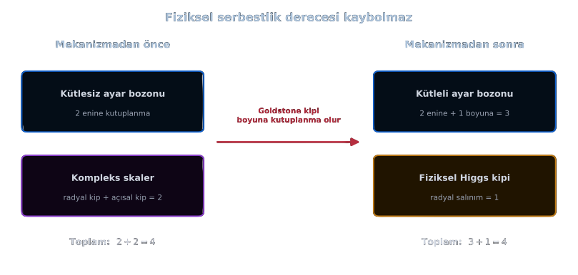
Before the mechanism, the massless vector has two transverse polarizations and the complex scalar has two real components, for a total of four. After the mechanism, the massive vector has three polarizations and the radial Higgs mode has one component: still four.

$$\underbrace{2}_{\text{kütlesiz vektör}} +\underbrace{2}_{\text{kompleks skaler}} = \underbrace{3}_{\text{kütleli vektör}} +\underbrace{1}_{\text{Higgs}}.$$

No physical degree of freedom has disappeared.

5.4 Unitary gauge is not the only choice: Rξ gauges

Unitary gauge makes the physical particle content transparent, but its high-momentum behavior can be inconvenient in loop calculations. With Cartesian variables,

$$\phi=\frac{1}{\sqrt{2}}(v+h+i\pi)$$

the quadratic Lagrangian density contains the mixing

$$gvA^\mu\partial_\mu\pi$$

We can cancel it using the gauge-fixing term

$$\mathcal L_{\mathrm{gf}} =-\frac{1}{2\xi} \left(\partial_\mu A^\mu-\xi gv\,\pi\right)^2$$

After integration by parts, the cross terms cancel and the Goldstone field appears to have the gauge-dependent mass

$$m_\pi^2=\xi m_A^2$$

This mass is not physical; it changes with $\xi$. Similarly, the unphysical part of the gauge-boson propagator depends on $\xi$. All $S$ dependence must cancel in an observable $\xi$-matrix element.

This distinction is extremely useful:

• Unitary gauge displays the physical spectrum intuitively.
• $R_\xi$ gauges organize renormalization and loop calculations.
• The conclusion: physical pole masses and cross sections are independent of the gauge choice.

In the Abelian example, Faddeev–Popov ghosts decouple from the physical sector. In a non-Abelian Higgs theory, ghost interactions are an integral part of the calculation.

6. Moving to the non-Abelian case: what does the mass matrix measure?

The electroweak group in the real world is non-Abelian. Even so, much of the geometry from the Abelian calculation survives unchanged. Consider a gauge group $G$ acting through generators $\Phi$ on a scalar multiplet $T^a$:

$$D_\mu\Phi =\left(\partial_\mu-i\sum_a g_aA_\mu^aT^a\right)\Phi.$$

Let the scalar field have the constant vacuum configuration

$$\langle\Phi\rangle=\Phi_0$$

The part of the kinetic term involving only the vacuum is

$$(D_\mu\Phi_0)^\dagger(D^\mu\Phi_0) = \sum_{a,b} g_ag_b A_\mu^aA^{b\mu} \Phi_0^\dagger T^aT^b\Phi_0$$

Because $A_\mu^aA^{b\mu}$ is symmetric under $a\leftrightarrow b$, we can write it using the anticommutator:

$$\mathcal L_{\mathrm{mass}} =\frac12A_\mu^a(M^2)_{ab}A^{b\mu}, \qquad \boxed{ (M^2)_{ab} =g_ag_b\, \Phi_0^\dagger\{T^a,T^b\}\Phi_0 }$$

The geometric meaning of this formula is especially clear. If a generator $T^a$ leaves the vacuum unchanged,

$$T^a\Phi_0=0,$$

there is a zero eigenvalue for the gauge field in that direction; the corresponding boson remains massless. Generators that change the vacuum are broken directions, and the corresponding gauge fields acquire nonzero eigenvalues in the mass matrix.

If the group $G$ is reduced to the subgroup $H$ that leaves the vacuum fixed,

$$G\longrightarrow H,$$

the number of broken generators is

$$\dim G-\dim H$$

In the generic regular case, the same number of would-be Goldstone modes become the longitudinal polarizations of massive gauge bosons. The remaining scalar components may be physical Higgs particles. In the minimal Higgs sector of the Standard Model, this counting is particularly elegant: three of the four real scalar components are used by $W^+$, $W^-$, and $Z$, while one remains as the physical Higgs boson.

7. The electroweak Higgs mechanism in the Standard Model

7.1 Field content and hypercharge convention

Let the electroweak gauge group be

$$G_{\mathrm{EW}}=SU(2)_L\times U(1)_Y$$

We denote the $SU(2)_L$ gauge fields by $W_\mu^a$ ($a=1,2,3$), and the $U(1)_Y$ gauge field by $B_\mu$. Their coupling constants are $g$ and $g'$, respectively.

The Higgs field is a complex $SU(2)_L$ doublet:

$$\Phi(x)= \begin{pmatrix} \phi^+(x)\\ \phi^0(x) \end{pmatrix}.$$

A complex doublet carries four real degrees of freedom. In this text, electric charge is defined by

$$Q=T^3+Y$$

and the Higgs doublet is assigned

$$Y_\Phi=\frac12$$

Thus the upper component has $T^3=+1/2$, since $Q=+1$, and the lower component has $T^3=-1/2$, since $Q=0$. Some sources write $Q=T^3+Y/2$ and take the Higgs hypercharge to be $Y_\Phi=1$. The physics is the same; only the normalization of the symbol $Y$ changes.

The covariant derivative is

$$D_\mu =\partial_\mu -ig\frac{\sigma^a}{2}W_\mu^a -ig'YB_\mu$$

and the Higgs Lagrangian density is

$$\mathcal L_{\mathrm{H}} =(D_\mu\Phi)^\dagger(D^\mu\Phi)-V(\Phi)$$

The most general renormalizable, electroweak-gauge-invariant scalar potential is

$$\boxed{ V(\Phi) =-\mu^2\Phi^\dagger\Phi +\lambda(\Phi^\dagger\Phi)^2, \qquad \mu^2,\lambda>0 }$$

The minimum condition gives

$$\Phi^\dagger\Phi=\frac{\mu^2}{2\lambda}\equiv\frac{v^2}{2}, \qquad v^2=\frac{\mu^2}{\lambda}$$

We choose the vacuum direction that preserves electric charge:

$$\boxed{ \langle\Phi\rangle =\frac{1}{\sqrt{2}} \begin{pmatrix} 0\\v \end{pmatrix}. }$$

Why give an expectation value to the neutral lower component rather than the upper one? If the vacuum carried electric charge, $U(1)_{\mathrm{em}}$ would also be in the Higgs phase and the photon would acquire mass. The long-range electromagnetism we observe tells us that the vacuum must satisfy $Q\langle\Phi\rangle=0$.

The electroweak scale fixed by the Fermi constant is

$$v=(\sqrt{2}G_F)^{-1/2}\simeq246\ \mathrm{GeV}$$

Here, $v$ is not a particle mass but the scale of the vacuum configuration.

7.2 Writing the Higgs doublet after symmetry breaking

In a general gauge, the doublet can be parametrized as

$$\Phi(x) =\exp\left[ \frac{i\xi^a(x)\sigma^a}{2v} \right] \frac{1}{\sqrt{2}} \begin{pmatrix} 0\\v+h(x) \end{pmatrix}$$

The three $\xi^a$ are the would-be Goldstone fields of the three broken directions. In unitary gauge, we set them to zero:

$$\Phi_{\mathrm{u}}(x) =\frac{1}{\sqrt{2}} \begin{pmatrix} 0\\v+h(x) \end{pmatrix}.$$

We will now read every mass from a single source, the term $(D_\mu\Phi)^\dagger(D^\mu\Phi)$.

7.3 The charged W± bosons

Use the Pauli matrices explicitly:

$$\sigma^1= \begin{pmatrix}0&1\\1&0\end{pmatrix}, \quad \sigma^2= \begin{pmatrix}0&-i\\i&0\end{pmatrix}, \quad \sigma^3= \begin{pmatrix}1&0\\0&-1\end{pmatrix}.$$

Acting on the vacuum,

$$\frac{\sigma^1}{2} \begin{pmatrix}0\\v/\sqrt{2}\end{pmatrix} =\frac{v}{2\sqrt{2}} \begin{pmatrix}1\\0\end{pmatrix}, \qquad \frac{\sigma^2}{2} \begin{pmatrix}0\\v/\sqrt{2}\end{pmatrix} =-\frac{iv}{2\sqrt{2}} \begin{pmatrix}1\\0\end{pmatrix}.$$

Thus the $W^1$ and $W^2$ fields excite the upper component. Define the physical charged combinations by

$$W_\mu^\pm =\frac{1}{\sqrt{2}} \left(W_\mu^1\mp iW_\mu^2\right)$$

The vacuum part of the kinetic term gives

$$\frac{g^2v^2}{8} \left[(W_\mu^1)^2+(W_\mu^2)^2\right] =\frac{g^2v^2}{4}W_\mu^+W^{-\mu}$$

For a complex vector field, the mass term is $m_W^2W_\mu^+W^{-\mu}$, so

$$\boxed{m_W=\frac{gv}{2}}.$$

The $W^+$ and $W^-$ are antiparticles of each other; as massive spin-1 particles, each has three polarizations.

7.4 The neutral sector: why do the Z and photon mix?

In the vacuum’s lower component, $T^3=-1/2$ and $Y=+1/2$, so the neutral covariant derivative is

$$D_\mu\langle\Phi\rangle \supset \frac{i v}{2\sqrt{2}} \left(gW_\mu^3-g'B_\mu\right) \begin{pmatrix}0\\1\end{pmatrix}$$

The neutral mass term is therefore

$$\mathcal L_{\mathrm{mass}}^{\mathrm{neutral}} =\frac{v^2}{8} \left(gW_\mu^3-g'B_\mu\right)^2$$

or, in matrix form,

$$\mathcal L_{\mathrm{mass}}^{\mathrm{neutral}} =\frac12 \begin{pmatrix}W_\mu^3&B_\mu\end{pmatrix} \frac{v^2}{4} \begin{pmatrix} g^2&-gg'\\ -gg'&g'^2 \end{pmatrix} \begin{pmatrix}W^{3\mu}\\B^\mu\end{pmatrix}$$

The determinant of the matrix vanishes:

$$\det \begin{pmatrix} g^2&-gg'\\ -gg'&g'^2 \end{pmatrix} =g^2g'^2-g^2g'^2=0.$$

Thus one eigenvalue is zero and the other is $g^2+g'^2$. Define the Weinberg angle by

$$\tan\theta_W=\frac{g'}{g}$$

and rotate to the mass eigenstates:

$$\boxed{ \begin{aligned} Z_\mu&=\cos\theta_W\,W_\mu^3-\sin\theta_W\,B_\mu,\\ A_\mu&=\sin\theta_W\,W_\mu^3+\cos\theta_W\,B_\mu. \end{aligned}}$$

This gives

$$\boxed{ m_Z=\frac{v}{2}\sqrt{g^2+g'^2}, \qquad m_\gamma=0 }$$

Electric charge also satisfies

$$\boxed{ e=g\sin\theta_W=g'\cos\theta_W }$$

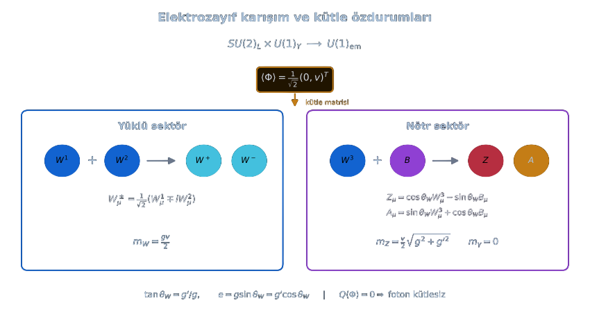
The photon remaining massless is not a coincidence, nor an extra assumption that the Higgs somehow “does not see” the photon. The generator that annihilates the vacuum is precisely the electromagnetic generator

$$Q=T^3+Y$$

Indeed,

$$Q\langle\Phi\rangle=0.$$

Consequently, $U(1)_{\mathrm{em}}$ remains the unbroken subgroup, and its gauge field $A_\mu$ corresponds to the zero eigenvalue of the mass matrix.

At tree level, the same calculation gives

$$\rho \equiv \frac{m_W^2}{m_Z^2\cos^2\theta_W} =1$$

This relation for the minimal Higgs doublet is one of the cornerstones of precision electroweak tests that constrain extended Higgs sectors.

7.5 What remains of the four scalar components?

Initially, the Higgs doublet carried four real components. The breaking pattern

$$SU(2)_L\times U(1)_Y \longrightarrow U(1)_{\mathrm{em}}$$

tells us that three of the four generators change the vacuum direction. The three would-be Goldstone fields provide the longitudinal polarizations of the $W^+$, $W^-$, and $Z$, respectively. One real scalar $h$ remains: the observed Higgs boson.

Write the potential using the doublet in unitary gauge:

$$\Phi^\dagger\Phi=\frac{(v+h)^2}{2}.$$

After using the minimum condition,

$$V(h) =\frac{\lambda}{4}\left[(v+h)^2-v^2\right]^2 =\lambda v^2h^2+\lambda vh^3+\frac{\lambda}{4}h^4.$$

Hence

$$\boxed{m_h^2=2\lambda v^2}$$

and the measured Higgs mass gives

$$\lambda=\frac{m_h^2}{2v^2}\approx0.13$$

Here we have used $m_h\simeq125.1\ \mathrm{GeV}$ and $v\simeq246\ \mathrm{GeV}$.

Writing the self-interactions with the normalization appropriate for Feynman rules,

$$\mathcal L \supset -\frac{1}{3!}\lambda_3h^3 -\frac{1}{4!}\lambda_4h^4$$

the Standard Model predicts

$$\boxed{ \lambda_3=\frac{3m_h^2}{v}, \qquad \lambda_4=\frac{3m_h^2}{v^2} }$$

An experimental measurement of the Higgs self-coupling tests not merely whether “we found a scalar,” but whether the potential really has the form of a Mexican hat.

7.6 The mass terms are also interaction terms

Because the covariant derivative contains $v+h$ in place of the vacuum, we obtain

$$m_W^2W_\mu^+W^{-\mu} \left(1+\frac{h}{v}\right)^2$$

and

$$\frac12m_Z^2Z_\mu Z^\mu \left(1+\frac{h}{v}\right)^2$$

Since

$$\left(1+\frac{h}{v}\right)^2 =1+\frac{2h}{v}+\frac{h^2}{v^2}$$

we have

$$\mathcal L \supset \frac{2m_W^2}{v}hW_\mu^+W^{-\mu} +\frac{m_Z^2}{v}hZ_\mu Z^\mu +\frac{m_W^2}{v^2}h^2W_\mu^+W^{-\mu} +\frac{m_Z^2}{2v^2}h^2Z_\mu Z^\mu.$$

Boson masses and Higgs-boson couplings are therefore not independent. They are different orders in the expansion of the same gauge-invariant term. This is why the strength of the Higgs interaction with the $W$ and $Z$ is proportional to the squared masses.

This relationship is experimentally crucial. It is not enough for a new scalar merely to appear as a resonance near $125\ \mathrm{GeV}$; it must exhibit the expected pattern of mass-dependent couplings to the $W$, $Z$, and fermions.

8. Fermions: how does the Yukawa interaction become mass?

8.1 The electron in one generation

We have already seen why a bare Dirac mass for the electron does not respect electroweak symmetry. The quantum numbers of the Higgs doublet are exactly what allow us to connect the left-handed doublet and the right-handed singlet in a gauge-invariant way:

$$\mathcal L_Y^{(e)} =-y_e\,\bar L_L\Phi\,e_R+\mathrm{h.c.}$$

Here,

$$L_L= \begin{pmatrix}\nu_{eL}\\e_L\end{pmatrix}.$$

In unitary gauge, substituting

$$\Phi=\frac{1}{\sqrt{2}} \begin{pmatrix}0\\v+h\end{pmatrix}$$

gives

$$\begin{aligned} \mathcal L_Y^{(e)} &=-\frac{y_e}{\sqrt{2}}(v+h)\bar e_Le_R+\mathrm{h.c.}\\ &=-\frac{y_ev}{\sqrt{2}}\bar e e -\frac{y_e}{\sqrt{2}}h\bar e e. \end{aligned}$$

Thus

$$\boxed{ m_e=\frac{y_ev}{\sqrt{2}}, \qquad \mathcal L_{hee}=-\frac{m_e}{v}h\bar e e. }$$

Again, the same structure gives two results: the vacuum part is the fermion mass, while the fluctuation part is the Higgs–fermion interaction. Since the tree-level coupling of the Higgs to a fermion is

$$g_{hff}=\frac{m_f}{v}$$

heavier fermions couple more strongly to the Higgs.

This statement should not be read in reverse: the Standard Model does not explain why the electron’s Yukawa coupling is $y_e\sim10^{-6}$ while that of the top quark is approximately one. We use the measured fermion masses to determine the Yukawa matrices. The Higgs mechanism explains how these numbers can appear as masses without breaking gauge symmetry.

8.2 Quarks, the conjugate doublet, and three generations

For down-type quarks, we can write

$$-\bar Q_LY_d\Phi\,d_R$$

Because up-type quarks have different hypercharges, we use the conjugate doublet

$$\widetilde\Phi \equiv i\sigma^2\Phi^\ast$$ $$-\bar Q_LY_u\widetilde\Phi\,u_R.$$

For all three generations,

$$\boxed{ \mathcal L_Y =-\bar Q_LY_d\Phi\,d_R -\bar Q_LY_u\widetilde\Phi\,u_R -\bar L_LY_e\Phi\,e_R +\mathrm{h.c.} }$$

Here $Y_u$, $Y_d$, and $Y_e$ are complex $3\times3$ matrices in family space. After symmetry breaking, the mass matrices are

$$M_f=\frac{v}{\sqrt{2}}Y_f$$

To diagonalize these matrices, we apply different unitary transformations to the left- and right-handed fields. If the left-handed transformations for the up- and down-type quarks differ, the charged current retains the mixing matrix

$$V_{\mathrm{CKM}}=U_{uL}^\dagger U_{dL}$$

Thus the Higgs sector and flavor physics meet within the same Yukawa structure.

8.3 Neutrinos and an important exception

The minimal Standard Model contains no right-handed neutrino field, so neutrinos are massless in the renormalizable Yukawa structure above. Oscillation experiments, however, show that at least two neutrinos have nonzero masses. This is direct evidence that physics beyond the minimal model is required.

Two common possibilities are:

1. Add right-handed neutrinos and generate Dirac masses with
   $-\bar L_LY_\nu\widetilde\Phi\,\nu_R$.
2. Use the dimension-five Weinberg operator:

$$\mathcal L_5 \sim \frac{c_{ij}}{\Lambda} \left(\bar L_i^c\widetilde\Phi^\ast\right) \left(\widetilde\Phi^\dagger L_j\right) +\mathrm{h.c.},$$

which, after inserting the vacuum, gives the approximate Majorana mass

$$m_\nu\sim\frac{cv^2}{\Lambda}$$

8.4 The misconception that “the Higgs is the source of all mass”

The mass parameters of elementary fermions such as the electron arise in the Lagrangian density through the Yukawa coupling and $v$. Most of the mass of ordinary matter, however, comes from protons and neutrons. A proton’s mass of approximately $938\ \mathrm{MeV}$ is not the simple sum of the bare masses of its two up quarks and one down quark; most of it is associated with QCD field energy, quark–gluon dynamics, and the trace anomaly.

Because the Higgs field determines the masses of light quarks, it makes an indirect and important contribution to the proton mass; nevertheless, it is wrong to say that “the Higgs gives all of the proton’s mass.” The precise achievement of the Higgs mechanism is to incorporate the mass terms of electroweak gauge bosons and elementary fermions into a gauge-invariant theory.

9. Longitudinal W scattering

Let us now see why the mechanism is necessary at high energy. For $E\gg m_W$, the longitudinal polarization vector of a massive spin-1 particle behaves roughly as

$$\epsilon_L^\mu(p) \simeq\frac{p^\mu}{m_W} +\mathcal O\left(\frac{m_W}{E}\right)$$

Because each external longitudinal $W$ leg can contribute a factor of order $E/m_W$, individual Feynman diagrams grow rapidly with energy. Gauge structure cancels many of the growing terms, but without the Higgs an $\mathcal O(E^2/v^2)$ behavior remains.

At high energy, the equivalence theorem relates amplitudes for longitudinal gauge bosons to those for the corresponding Goldstone fields:

$$\mathcal M(W_L^a\cdots) =\mathcal M(\pi^a\cdots) +\mathcal O\left(\frac{m_W}{E}\right).$$

If we remove the Higgs from the effective theory and retain only the electroweak Goldstone modes, the leading amplitude for, say,

$$\pi^+\pi^-\to\pi^0\pi^0$$

is

$$\mathcal M(s,t,u)\simeq\frac{s}{v^2}$$

The $J=0$ partial wave is then

$$\begin{aligned} a_0(s) &=\frac{1}{32\pi} \int_{-1}^{1}d(\cos\theta)\,\mathcal M(s,\theta)\\ &=\frac{s}{16\pi v^2} \end{aligned}$$

Perturbative unitarity for elastic scattering requires, roughly,

$$|\operatorname{Re}a_0|\le\frac12$$

Therefore,

$$\sqrt{s} \lesssim \sqrt{8\pi}\,v \simeq1.2\ \mathrm{TeV}.$$

This does not mean that “the theory definitely ends at $1.2\ \mathrm{TeV}$”; channel mixing and a detailed partial-wave analysis alter the numerical coefficients. It means that, without the Higgs or other new dynamics providing the same cancellation, weak-boson scattering becomes strongly coupled at the TeV scale.

When the Standard Model Higgs is included, $h$ exchange cancels the $s/v^2$ term that grows at high energy. Schematically,

$$\mathcal M_{\mathrm{gauge}} \sim\frac{s}{v^2}, \qquad \mathcal M_h \sim-\frac{s}{v^2} +\mathcal O\left(\frac{m_h^2}{v^2}\right),$$

and the total amplitude approaches a constant rather than growing with energy. For this cancellation to work, the $hWW$ and $hZZ$ coupling coefficients must have exactly the values implied by the mass terms.

Observing the Higgs boson is therefore not merely “finding the particle of the field that gives mass.” It tests the network of amplitudes that keeps the electroweak theory unitary and perturbative at high energy.

10. Conclusion

We can now summarize the Higgs mechanism more accurately in a single sentence:

When the gauge-invariant potential of a scalar field selects a nonzero vacuum scale, the covariant derivative generates mass terms for certain gauge fields around that vacuum; the would-be Goldstone modes provide the longitudinal polarizations of the massive vectors, while the radial excitation remains as the physical Higgs boson.

We have now given the Higgs mechanism the account it deserves. Thank you for reading.
See you in the other articles :)

References

1. J. Goldstone, A. Salam and S. Weinberg, “Broken Symmetries”, Physical Review 127, 965 (1962). DOI: 10.1103/PhysRev.127.965
2. P. W. Anderson, “Plasmons, Gauge Invariance, and Mass”, Physical Review 130, 439 (1963). DOI: 10.1103/PhysRev.130.439
3. F. Englert and R. Brout, “Broken Symmetry and the Mass of Gauge Vector Mesons”, Physical Review Letters 13, 321 (1964). DOI: 10.1103/PhysRevLett.13.321
4. P. W. Higgs, “Broken Symmetries, Massless Particles and Gauge Fields”, Physics Letters 12, 132 (1964). DOI: 10.1016/0031-9163(64)91136-9
5. P. W. Higgs, “Broken Symmetries and the Masses of Gauge Bosons”, Physical Review Letters 13, 508 (1964). DOI: 10.1103/PhysRevLett.13.508
6. G. S. Guralnik, C. R. Hagen and T. W. B. Kibble, “Global Conservation Laws and Massless Particles”, Physical Review Letters 13, 585 (1964). DOI: 10.1103/PhysRevLett.13.585
7. T. W. B. Kibble, “Symmetry Breaking in Non-Abelian Gauge Theories”, Physical Review 155, 1554 (1967). DOI: 10.1103/PhysRev.155.1554
8. S. Weinberg, “A Model of Leptons”, Physical Review Letters 19, 1264 (1967). DOI: 10.1103/PhysRevLett.19.1264
9. S. Elitzur, “Impossibility of Spontaneously Breaking Local Symmetries”, Physical Review D 12, 3978 (1975). DOI: 10.1103/PhysRevD.12.3978
10. D. Tong, Lectures on the Standard Model, Part 2: Broken Symmetries (Cambridge, 2019-2024). Lecture notes
11. Particle Data Group, “Status of Higgs Boson Physics”, Review of Particle Physics, 2025 update. PDG review (PDF)
12. ATLAS Collaboration, “Observation of a New Particle in the Search for the Standard Model Higgs Boson with the ATLAS Detector at the LHC”, Physics Letters B 716, 1 (2012). arXiv:1207.7214
13. CMS Collaboration, “Observation of a New Boson at a Mass of 125 GeV with the CMS Experiment at the LHC”, Physics Letters B 716, 30 (2012). arXiv:1207.7235
14. ATLAS and CMS Collaborations, “Combined Measurement of the Higgs Boson Mass in $pp$ Collisions at $\sqrt{s}=7$ and $8\ \mathrm{TeV}$”, Physical Review Letters 114, 191803 (2015). DOI: 10.1103/PhysRevLett.114.191803