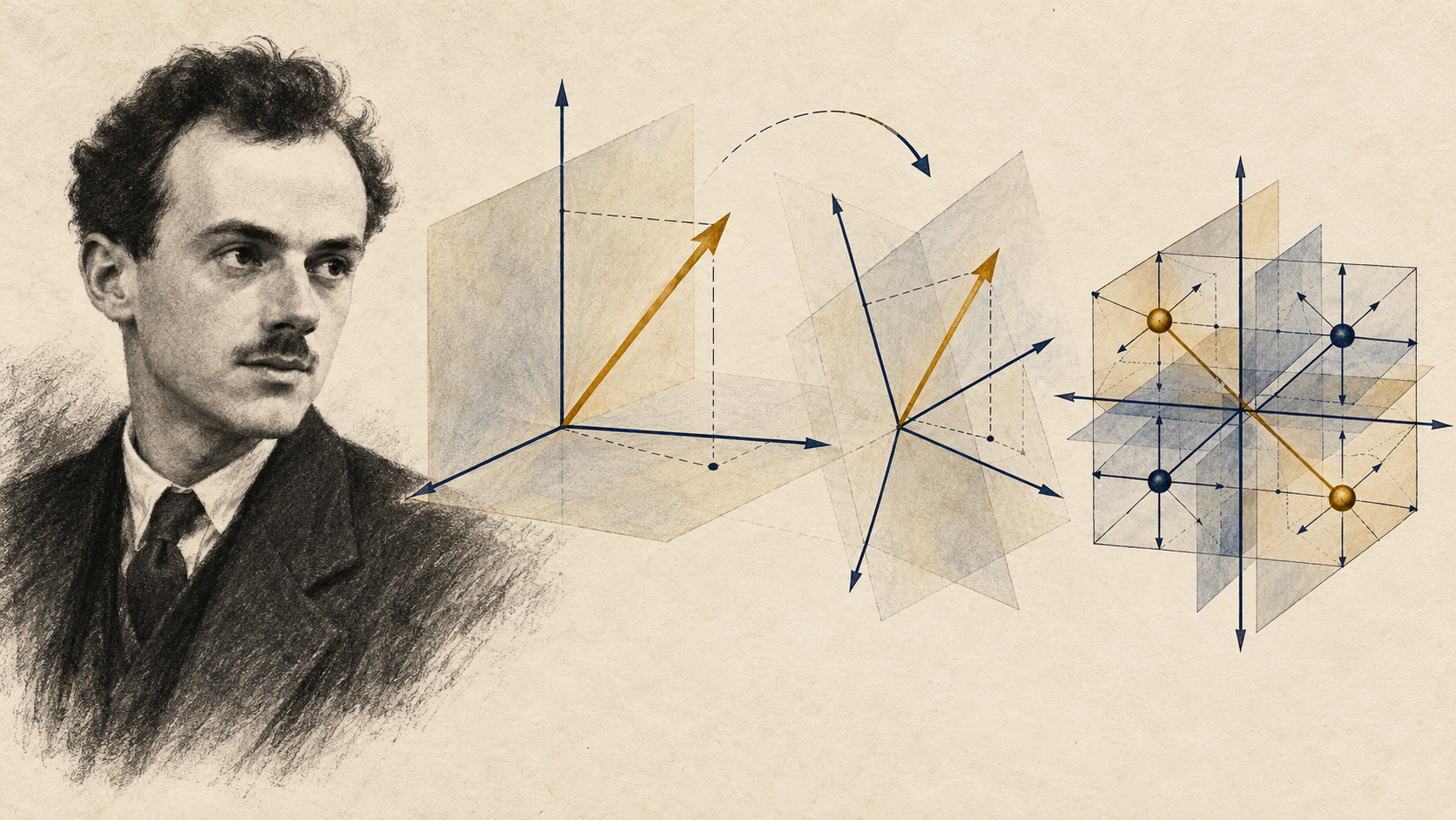
The Heart of Quantum Mechanics: Linear Algebra and Bra-Ket Notation

The Heart of Quantum Mechanics: Linear Algebra and Bra-Ket Notation

[!quote] “It troubles me greatly that, in quantum theory, which we accept as a good theory, we neglect infinities. This is not sensible. In mathematics, sensibly, you neglect a quantity because it is very small — not because it is infinitely large and you do not want it.”

— A rendering of Paul Dirac’s criticism of renormalization [1]

For Paul Dirac, the mathematical beauty of physical laws was an important guide in the construction of theories [2]. Yet the relationship between mathematical elegance and an accurate description of nature is not always free of tension. When infinite quantities appear in the calculations of a theory, how should they be handled? Can a theory that agrees remarkably well with experiment still be judged incomplete in its mathematical structure?

Dirac’s unease with renormalization is one historical instance of these questions. The infinities at issue here are a different matter from the measurement uncertainties of quantum mechanics: they are mathematical divergences that arise in certain calculations of quantum field theory.

The mathematical elegance Dirac sought, on the other hand, finds one of its strongest expressions in quantum mechanics through linear algebra. Even where our everyday intuitions fall short, vector spaces, inner products and operators allow physical predictions to be computed clearly and consistently. While debates over the interpretation of quantum mechanics continue, this mathematical structure goes on producing results that can be compared with experiment.

How Do We Define Linear Algebra?

In mathematics, linear algebra is the branch that studies vector spaces, linear maps and the representation of these maps by matrices. Its range of applications is broad, extending from the solution of systems of linear equations to geometric transformations, and from numerical computation to abstract mathematical structures.

The linear algebra used in quantum mechanics is not a separate algebra from that of mathematics. The difference lies in the physical purpose for which the same structures are used and in how they are interpreted.

The Role of Linear Algebra in Mathematics

• Focus: Vector spaces, linear maps, matrices, eigenvalues, determinants and systems of linear equations.
• Number systems: One may work over the real numbers $\mathbb{R}$, the complex numbers $\mathbb{C}$, or more general fields.
• Dimension: Both finite- and infinite-dimensional vector spaces may be considered. In infinite dimensions, issues such as continuity, convergence and the domains of operators also become important.
• Aim: To understand geometric relationships, to carry out computations and to develop general mathematical results.

Linear Algebra in Quantum Mechanics

In quantum mechanics, these structures are used to describe physical states and how they change.

Hilbert space: State vectors are defined in a complex Hilbert space. A Hilbert space is an inner product space that is complete with respect to the norm induced by the inner product. Completeness here means that every sequence of vectors that is Cauchy with respect to this norm has a limit that again lies in the space [3, 5].

Dirac notation: Bra and ket symbols are used to express abstract vectors and the relations between them [9]:

• $|v\rangle$, the ket, denotes an abstract vector in the Hilbert space. Once an orthonormal basis is chosen, the components of this vector can be represented by a column vector.

• $\langle f|$, the bra, is the continuous linear functional that corresponds to the ket $|f\rangle$ via the inner product. In the matrix representation with respect to the chosen orthonormal basis, it is represented by the conjugate transpose of the ket: $\langle f| = (|f\rangle)^\dagger$.

  Here $\dagger$ denotes complex conjugation and transposition taken together. The correspondence between kets and their bras is antilinear.

• $\langle f|v\rangle$ is the inner product of two vectors and is a complex number. For normalized states, in an appropriate measurement context, it can be interpreted as a probability amplitude [3, 5].

Operators: Linear maps acting on the state space.

• Self-adjoint operators represent observable quantities such as position, momentum and energy in standard quantum mechanics. Their spectra are real.
• Unitary operators represent the time evolution of a closed system given by the Schrödinger equation, as well as many symmetry transformations. They preserve inner products and hence norms: $U^\dagger U = UU^\dagger = I$.

In finite-dimensional spaces the terms Hermitian and self-adjoint express the same condition. In infinite-dimensional spaces, however, domains matter, particularly for unbounded operators: being symmetric is not by itself sufficient for being self-adjoint. For this reason, we shall use the condition of self-adjointness in the general mathematical definition of observables.

Reading the Postulates of Quantum Mechanics in the Language of Linear Algebra

The rules of quantum mechanics are built on physical postulates adopted in order to account for experimental facts. Linear algebra does not derive these postulates on its own; it makes it possible to express them mathematically and to compute their consequences.

When states, probabilities, measurements and time evolution are brought together within the same geometric framework, strong connections emerge among quantum phenomena that at first sight appear unrelated.

1. States and the Structure of Hilbert Space

Superposition → State vectors and rays

Quantum phenomenon: In accordance with the superposition principle, quantum states can be expressed as linear combinations.

Linear-algebraic counterpart: This linear structure is provided by the Hilbert space $\mathcal{H}$ in which state vectors are defined. Physical pure states, however, are represented not by a single vector in this space but by a ray, that is, a one-dimensional subspace.

For example, the normalized vectors

$$|\psi\rangle \quad \text{and} \quad e^{i\theta}|\psi\rangle$$

represent the same physical pure state. The global phase difference between them does not change measurement probabilities.

Physical states themselves do not form a vector space under addition and scalar multiplication. For a normalized $|\psi\rangle$, the vector $2|\psi\rangle$ is not normalized; moreover, the vector

$$|\psi\rangle - |\psi\rangle = 0$$

does not specify a physical state.

By contrast, thanks to the linear structure of the underlying Hilbert space, combinations such as

$$c_1|a\rangle + c_2|b\rangle$$

can be formed. If this combination is nonzero, it can be normalized to give a new state vector. Where the superposition is physically realizable, this vector represents a new pure state.

More general states, including statistical mixtures, are described by density operators $\rho$ [5].

2. Probability and the Inner Product Space

The Born rule → The inner product and the Cauchy–Schwarz inequality

Quantum phenomenon: Measurement outcomes are described by probabilities, and the total probability of all mutually exclusive possible outcomes is 1.

Linear-algebraic counterpart: Probability amplitudes are related to inner products, and the total-probability condition to normalization:

$$|\psi|^2 = \langle\psi|\psi\rangle = 1.$$

For a normalized state $|\psi\rangle$, the probability of the projective measurement outcome associated with the one-dimensional subspace determined by the normalized vector $|\phi\rangle$ is given by

$$p = |\langle\phi|\psi\rangle|^2.$$

The Cauchy–Schwarz inequality ensures that the squared modulus of the inner product does not exceed 1:

$$|\langle\phi|\psi\rangle|^2 \le \langle\phi|\phi\rangle\langle\psi|\psi\rangle = 1.$$

Thus the quantity interpreted as a probability through the Born rule remains, mathematically, within the interval $[0, 1]$ for normalized states [5, 6].

3. Observation and Measurement

Observables → The spectral theorem

Quantum phenomenon: The measurement outcomes of an observable are related to the spectral structure of the operator that represents it.

Linear-algebraic counterpart: In finite dimensions this structure appears through the eigenvalue–eigenvector problem:

$$A|v\rangle = \lambda|v\rangle.$$

In the standard projective measurement formalism, observables are represented by self-adjoint operators. The spectral theorem allows these operators to be associated with real measurement outcomes and with the projection operators belonging to those outcomes.

In finite dimensions, an orthonormal basis can be chosen from the eigenvectors of a Hermitian operator. In infinite dimensions, a continuous spectrum may also be present, and the description requires a spectral measure more general than ordinary sums over eigenvectors.

In an ideal projective measurement with discrete spectrum, an eigenvalue is obtained and the state is updated by projecting it onto the corresponding eigenspace. In the continuous spectrum, by contrast, not every spectral value need have a normalizable eigenvector. For instance, the ideal position kets $|x\rangle$ are not ordinary vectors of the $L^2$ space in which physical states live. The probabilities of a position measurement can be expressed in terms of finite position intervals.

The importance of self-adjointness is not merely that the eigenvalues are real. An operator with real eigenvalues is not necessarily self-adjoint. The required structure is provided by the spectral decomposition, which defines the measurement outcomes and their probabilities together [5, 6, 12].

4. The Outer Product and Projection Operators

Projectors → The resolution of the identity

Quantum phenomenon: The outcome obtained in an ideal projective measurement determines how the state is to be updated.

Linear-algebraic counterpart: Projection operators. The projection onto the one-dimensional subspace spanned by a normalized vector $|i\rangle$ is denoted

$$\Pi_i = |i\rangle\langle i|.$$

The outer product of a ket and a bra,

$$|u\rangle\langle v|,$$

produces an operator. Its action on an arbitrary vector $|\psi\rangle$ is

$$(|u\rangle\langle v|)|\psi\rangle = |u\rangle\langle v|\psi\rangle:$$

first the complex number $\langle v|\psi\rangle$ is computed, and then $|u\rangle$ is multiplied by this number.

Not every outer product is a projector. When $|i\rangle$ is normalized, $|i\rangle\langle i|$ is an orthogonal projector and satisfies

$$\Pi_i^\dagger = \Pi_i, \qquad \Pi_i^2 = \Pi_i.$$

For a complete orthonormal basis ${|i\rangle}$, the identity operator resolves as

$$\sum_i |i\rangle\langle i| = I.$$

Consequently, any state vector can be written as

$$|\psi\rangle = I|\psi\rangle = \sum_i |i\rangle\langle i|\psi\rangle = \sum_i c_i|i\rangle, \qquad c_i = \langle i|\psi\rangle.$$

This relation is the Dirac-notation counterpart of decomposing a vector into its components in a chosen basis [3, 5, 10].

From Popular Exposition to Abstract Algebra: Odenwald’s Analysis of Quantum States

In introductory texts on quantum mechanics, the measurement problem is often approached in intuitive and philosophical language. The relationship between superposition and measurement discussed in Sten Odenwald’s book on quantum physics is one example of this approach [4].

We might think that looking at an object in the everyday world does not visibly change it. Physical measurement, however, requires an interaction between the system and the measuring apparatus. While the effects of this interaction are often negligible under macroscopic conditions, in quantum systems the nature of the measured quantity and of the prepared state is decisive.

The important distinction here is this: a system is described by a quantum state even before measurement; but this state need not correspond to a definite value of the observable being measured.

Let us write the state of an electron, in a chosen orthonormal basis, as

$$|\Psi\rangle = \sum_i a_i|\phi_i\rangle = a_1|\phi_1\rangle + a_2|\phi_2\rangle + a_3|\phi_3\rangle + \cdots$$

Here $|\phi_i\rangle$ are basis vectors and $a_i$ are complex probability amplitudes. When the measurement is defined by the one-dimensional projectors of this basis,

$$p_i = a_i^* a_i = |a_i|^2$$

gives the probability of the corresponding outcome.

When a definite state is obtained as the result of a measurement, what becomes of the other amplitudes and phase relations present in the initial superposition? Dirac notation expresses clearly the part of this question that concerns the measurement rule; it does not, however, resolve all the physical and interpretive dimensions of the measurement problem on its own.

Amplitude as an inner product: The coefficient in the expansion is the component of the state vector along the basis vector:

$$a_i = \langle\phi_i|\Psi\rangle.$$

The Born probability is the squared modulus of this component:

$$p_i = |\langle\phi_i|\Psi\rangle|^2.$$

Measurement and state update: In an ideal measurement with discrete spectrum, if the eigenvalue associated with outcome $i$ is nondegenerate, then

$$\Pi_i = |\phi_i\rangle\langle\phi_i|.$$

If more than one linearly independent eigenvector corresponds to the same eigenvalue, the projection onto the corresponding eigenspace is given by

$$\Pi_i = \sum_k |\phi_{i,k}\rangle\langle\phi_{i,k}|.$$

For a normalized initial state, the probability of the outcome and the conditional state update according to the Lüders rule are:

$$p_i = \langle\Psi|\Pi_i|\Psi\rangle, \qquad |\Psi_i\rangle = \frac{\Pi_i|\Psi\rangle}{\sqrt{p_i}}, \qquad p_i > 0.$$

In the nondegenerate case,

$$|\Psi_i\rangle = \frac{a_i}{|a_i|}|\phi_i\rangle$$

is obtained. The leading coefficient is merely a global phase; hence the new physical state is represented by $|\phi_i\rangle$.

In the degenerate case, by contrast, the system remains in the corresponding eigenspace; in general it is not reduced to a single, previously chosen basis vector. This update describes an ideal Lüders measurement. The effects on the state of more detailed or different physical setups measuring the same observable must be specified separately [7].

The geometry of projection shows how the state is updated once an outcome has been obtained. Which particular outcome occurs, and how to interpret a description in which system and apparatus are treated together, belong to the measurement problem.

Projective measurements are not the only kind of measurement. In a more general setting where each outcome is represented by a single measurement operator $M_m$, the condition

$$\sum_m M_m^\dagger M_m = I$$

holds. For a pure initial state one writes

$$p_m = \langle\Psi|M_m^\dagger M_m|\Psi\rangle, \qquad |\Psi_m\rangle = \frac{M_m|\Psi\rangle}{\sqrt{p_m}};$$

the state update applies to outcomes with $p_m > 0$.

The operators

$$E_m = M_m^\dagger M_m$$

are the elements of a POVM, a positive operator-valued measure. The POVM determines the probabilities of the outcomes; to determine the post-measurement state, additional information about how the measurement is implemented on the system is required.

More generally, more than one measurement operator may correspond to the same recorded outcome. In such a case, a conditionally mixed state may be obtained even from a pure initial state [7].

Normalization condition: The requirement that the total probability of all mutually exclusive outcomes be 1,

$$\sum_i p_i = 1,$$

is related, in a complete orthonormal basis, to the state vector having unit norm:

$$\langle\Psi|\Psi\rangle = 1.$$

5. The Flow of Time and Symmetries

Time evolution → Unitary operators

Quantum phenomenon: Total probability is conserved in the Schrödinger evolution of a closed system.

Linear-algebraic counterpart: Unitary transformations:

$$U^\dagger U = UU^\dagger = I.$$

Unitary operators preserve the norms of vectors and the inner products between them. In this sense, quantum evolution can be thought of as a transformation in Hilbert space that preserves lengths and geometric relations. The geometry here is not that of everyday three-dimensional space but that of the complex state space [5].

The time evolution of a system is written as

$$|\psi(t)\rangle = U(t, t_0)|\psi(t_0)\rangle.$$

When the Hamiltonian is time-independent,

$$U(t, t_0) = e^{-\frac{i}{\hbar}H(t - t_0)}$$

is obtained. In this case the evolution depends only on the elapsed time. Stone’s theorem states that strongly continuous one-parameter unitary groups have a self-adjoint generator; in quantum mechanics this generator, up to the appropriate factor of $\hbar$, is the Hamiltonian.

If the Hamiltonian depends explicitly on time, the evolution is in general expressed as

$$U(t, t_0) = \mathcal{T}\exp\left[-\frac{i}{\hbar}\int_{t_0}^{t} H(s),ds\right].$$

Here $\mathcal{T}$ time-orders products of Hamiltonians at different times. This is necessary because, in general, $H(t_1)$ and $H(t_2)$ do not commute [16].

The same mathematical idea extends to symmetries. According to Wigner’s theorem, appropriate symmetry transformations that preserve transition probabilities between pure states are represented on Hilbert space by unitary or antiunitary operators. Time-reversal symmetry is an important example of an antiunitary representation.

The generator of spatial translations is momentum; the generator of rotations is angular momentum. For an observable $G$ with no explicit time dependence, the condition

$$[H, G] = 0$$

ensures that the corresponding quantity is conserved under time evolution. If there is also explicit time dependence, the rate of change of the expectation value is determined by

$$\frac{d}{dt}\langle G\rangle = \frac{i}{\hbar}\langle[H, G]\rangle + \left\langle\frac{\partial G}{\partial t}\right\rangle.$$

In this way, the concepts of symmetry, conservation law and operator are unified within the same mathematical framework.

From Abstract Geometry to Physical Intuition: Visualizing the Quantum World

Mathematical axioms and Dirac notation may seem abstract at first sight. But when we consider the basic concepts together with geometric analogies, the physical meaning of these structures becomes easier to grasp. The value of an analogy lies in seeing at once what it explains and where it falls short.

1. State Space and Directions: A World of Arrows

In everyday life we describe a light switch as either on or off. The state of a two-level quantum system, however, does not have to be one of the two basis states.

Imagine that, on the floor of a room, the forward direction represents the state $|0\rangle$ and the rightward direction the state $|1\rangle$. An arrow pointing diagonally between these two axes can be a first step toward visualizing superposition.

This analogy, however, has an important limitation: Hilbert space is defined over the complex numbers. The physical properties of states therefore depend not only on the magnitudes of the amplitudes but also on the relative phases between them.

For example, the states

$$|+\rangle = \frac{|0\rangle + |1\rangle}{\sqrt{2}}, \qquad |-\rangle = \frac{|0\rangle - |1\rangle}{\sqrt{2}}$$

give the same measurement probabilities in the ${|0\rangle, |1\rangle}$ basis. In both cases the outcome 0 or 1 is obtained with probability $1/2$.

Nevertheless, these two states are orthogonal:

$$\langle +|-\rangle = 0.$$

An ideal measurement in the ${|+\rangle, |-\rangle}$ basis can distinguish these states with certainty. The relative phase shows up in observable results when the measurement basis is changed.

The dimension of the state space depends on which physical degrees of freedom are being modeled. The spin state alone of a spin-$\frac{1}{2}$ particle is described in a two-dimensional space. If the particle’s motion in space is also taken into account, the state space is, for example,

$$\mathcal{H} = L^2(\mathbb{R}^3) \otimes \mathbb{C}^2.$$

Here $L^2(\mathbb{R}^3)$ carries the spatial wavefunctions and $\mathbb{C}^2$ the spin components.

One natural way to visualize the pure states of two-level systems is the Bloch sphere. The normalized pure state of a qubit can be written, up to a global phase, as

$$|\psi\rangle = \cos\frac{\theta}{2}|0\rangle + e^{i\phi}\sin\frac{\theta}{2}|1\rangle, \qquad 0 \le \theta \le \pi, \quad 0 \le \phi < 2\pi.$$

These angles determine a point on the unit sphere. $|0\rangle$ lies at the north pole and $|1\rangle$ at the south pole. $|+\rangle$ and $|-\rangle$ correspond to antipodal points on the equator.

On the Bloch sphere, antipodal points represent orthogonal states in Hilbert space. Hence the geometric angle on the sphere is not the same as the angle between kets; the half-angle in the expression for the state reflects this relationship.

Pure states lie on the surface of the sphere, while mixed states lie in its interior. This representation is specific to two-level systems [7].

Making Bra-Ket Notation Concrete: A Two-Level Example

Consider the normalized state

$$|\psi\rangle = \frac{\sqrt{3}}{2}|0\rangle + \frac{1}{2}|1\rangle.$$

Choosing the orthonormal basis ${|0\rangle, |1\rangle}$,

$$|0\rangle = \begin{pmatrix} 1 \ 0 \end{pmatrix}, \qquad |1\rangle = \begin{pmatrix} 0 \ 1 \end{pmatrix}$$

and

$$|\psi\rangle = \begin{pmatrix} \sqrt{3}/2 \ 1/2 \end{pmatrix}.$$

The corresponding bra is

$$\langle\psi| = \begin{pmatrix} \sqrt{3}/2 & 1/2 \end{pmatrix}.$$

Since the coefficients are real in this example, complex conjugation leaves them unchanged.

Let us compute the norm:

$$\langle\psi|\psi\rangle = \frac{3}{4} + \frac{1}{4} = 1.$$

The measurement probabilities in the standard basis are found to be

$$p_0 = |\langle 0|\psi\rangle|^2 = \frac{3}{4}, \qquad p_1 = |\langle 1|\psi\rangle|^2 = \frac{1}{4}.$$

If the outcome 0 is obtained in the measurement,

$$\Pi_0|\psi\rangle = |0\rangle\langle 0|\psi\rangle = \frac{\sqrt{3}}{2}|0\rangle.$$

Dividing this vector by $\sqrt{p_0} = \sqrt{3}/2$ yields the normalized post-measurement state $|0\rangle$.

Now let us measure the same initial state in the ${|+\rangle, |-\rangle}$ basis:

$$\langle +|\psi\rangle = \frac{\sqrt{3} + 1}{2\sqrt{2}}, \qquad \langle -|\psi\rangle = \frac{\sqrt{3} - 1}{2\sqrt{2}}.$$

Thus

$$p_+ = \frac{2 + \sqrt{3}}{4}, \qquad p_- = \frac{2 - \sqrt{3}}{4},$$

and once again $p_+ + p_- = 1$.

The initial state has not changed; what has changed is which measurement is performed. Bra-ket notation keeps this distinction explicit by displaying the state vector and the measurement basis separately.

2. Measurement and Wavefunction Collapse: The Lantern-and-Shadow Metaphor

We can think about the geometric side of ideal projective measurement through a shadow analogy.

Let a thin rod standing diagonally in space represent the state vector. The shadow cast by parallel light can help us visualize a projection onto a plane. To think of a one-dimensional projector, however, we must focus on the component of this shadow that remains along a chosen axis.

The projection onto the direction of a normalized $|i\rangle$ is given by

$$\Pi_i|\psi\rangle = |i\rangle\langle i|\psi\rangle.$$

The squared norm of this projection is the probability of the corresponding measurement outcome:

$$p_i = |\Pi_i|\psi\rangle|^2.$$

The state after the outcome is obtained is not the projection itself but its renormalized form:

$$|\psi_i\rangle = \frac{\Pi_i|\psi\rangle}{\sqrt{p_i}}, \qquad p_i > 0.$$

The limitation of the analogy matters here: a classical shadow does not explain which outcome of a quantum measurement will occur. The geometry of projection shows how the state is updated conditional on a given outcome. The occurrence of individual outcomes and the role of the measuring apparatus are the subject of the broader measurement problem.

3. Order Matters: Why Are $AB$ and $BA$ Not the Same?

When multiplying two ordinary numbers, order does not matter:

$$2 \times 3 = 3 \times 2.$$

For linear maps, by contrast, in general

$$AB \neq BA.$$

We can picture this with an everyday example: putting on socks and then shoes does not give the same result as doing these operations in the reverse order. This example is not a model of quantum measurement; it only shows that the order of operations can change the result.

In quantum mechanics, observables are represented by operators. The effects of successive measurements, in turn, depend on the state-update rules of the measurements involved. For measurements of observables that do not commute with each other, the order can affect the statistics of the outcomes.

The fundamental relation for position and momentum is

$$[X, P] = XP - PX = i\hbar I.$$

One quantitative expression of the uncertainty principle is the Robertson inequality:

$$\Delta A,\Delta B \ge \frac{1}{2}\left|\langle[A, B]\rangle\right|.$$

Here

$$\Delta A = \sqrt{\langle A^2\rangle - \langle A\rangle^2}$$

is the standard deviation in the given state. The relation is used in cases where the required expectation values and operator expressions are well defined.

Substituting the commutator of position and momentum gives

$$\Delta X,\Delta P \ge \frac{\hbar}{2}.$$

This relation constrains the spreads of the position and momentum distributions in identically prepared systems; it is not merely an error relation arising from imperfections of measuring devices.

Operators that do not commute may still share some common eigenvectors. For Hermitian operators in finite dimensions, however, the existence of a common orthonormal eigenbasis spanning the whole space requires the operators to commute. In infinite dimensions, the formulation of this relationship must also take into account domains and spectral projectors.

Moreover, no finite-dimensional matrices satisfy the relation $[X, P] = i\hbar I$. This is because, in finite dimensions, the trace of a commutator is zero:

$$\operatorname{Tr}(XP - PX) = 0,$$

whereas in $n$ dimensions

$$\operatorname{Tr}(i\hbar I) = i\hbar n.$$

This contradiction shows why the canonical position and momentum operators are treated in an infinite-dimensional setting.

Combining Systems: The Tensor Product and Quantum Entanglement

So far we have considered the state space of a single system. Physical systems, however, come together, interact and form joint states. To describe several subsystems together, one of the fundamental structures of linear algebra is used: the tensor product.

The Tensor Product and Kronecker Notation in Linear Algebra

The tensor product of two vector spaces,

$$V \otimes W,$$

combines vectors belonging to these spaces within a structure that is linear in each argument. Its counterpart for matrices and column vectors in chosen bases is the Kronecker product [7, 11].

In the Kronecker product, each entry of the left-hand matrix multiplies the entire right-hand matrix to form a block. For example,

$$\begin{pmatrix} a \ b \end{pmatrix} \otimes \begin{pmatrix} c \ d \end{pmatrix} = \begin{pmatrix} ac \ ad \ bc \ bd \end{pmatrix}.$$

If the finite-dimensional spaces $V$ and $W$ have dimensions $m$ and $n$ respectively, then

$$\dim(V \otimes W) = mn.$$

The dimension of the joint space is not the sum but the product of the dimensions of the subsystem spaces.

Its Place in Quantum Mechanics: Combining State Spaces

The joint state space of two distinguishable subsystems is constructed as

$$\mathcal{H}_{\text{total}} = \mathcal{H}_A \otimes \mathcal{H}_B.$$

A single qubit is described in a two-dimensional Hilbert space. The joint space of two qubits is four-dimensional, and its standard orthonormal basis is

$${|00\rangle, |01\rangle, |10\rangle, |11\rangle}.$$

Here the shorthand

$$|00\rangle = |0\rangle \otimes |0\rangle$$

is used.

The tensor-product structure remains important for identical particles as well; however, physical states must satisfy the appropriate symmetry conditions under particle exchange. The symmetric subspace is used for bosons and the antisymmetric subspace for fermions.

For $N$ distinguishable subsystems, each with two levels, the dimension of the joint Hilbert space is

$$2^N.$$

This expression holds not for a general $N$-particle system but for the $N$-qubit structure considered here.

Exponential growth in dimension does not by itself guarantee a computational advantage. A single measurement cannot read out all $2^N$ complex amplitudes of the state. Quantum algorithms are designed to exploit interference between amplitudes so as to make it easier to obtain the desired results for particular computational problems. Shor’s and Grover’s algorithms are important examples of quantum speedup under different problems and comparison conditions [7].

Single-qubit operations applied independently to the subsystems combine in the form

$$A \otimes B.$$

A two-qubit gate capable of generating entanglement, by contrast, cannot be reduced to a single product of independent local operations.

For example, the controlled-NOT gate is written as

$$\text{CNOT} = |0\rangle\langle 0| \otimes I + |1\rangle\langle 1| \otimes X.$$

Here $X$ is the Pauli operator that interchanges the states $|0\rangle$ and $|1\rangle$.

If the first qubit is in the state $|0\rangle$, the identity is applied to the second qubit; if the first qubit is in the state $|1\rangle$, the second qubit is flipped. This gate cannot be written as a single product $A \otimes B$, and it can generate entangled states from suitable initial states.

Quantum Entanglement: States That Cannot Be Factorized

Not every vector in the tensor-product space is a single product vector. Some pure states cannot be written in the form

$$|\psi_A\rangle \otimes |\psi_B\rangle.$$

Such states are called entangled pure states.

Consider one of the Bell states:

$$|\Phi^+\rangle = \frac{|00\rangle + |11\rangle}{\sqrt{2}}.$$

Suppose this state could be written as a product of two single-qubit states:

$$(c_1|0\rangle + c_2|1\rangle) \otimes (d_1|0\rangle + d_2|1\rangle).$$

Expanding the product gives

$$c_1 d_1|00\rangle + c_1 d_2|01\rangle + c_2 d_1|10\rangle + c_2 d_2|11\rangle.$$

For this to equal $|\Phi^+\rangle$, we would need

$$c_1 d_1 = c_2 d_2 = \frac{1}{\sqrt{2}}, \qquad c_1 d_2 = c_2 d_1 = 0.$$

The first conditions require all of the coefficients $c_1, c_2, d_1, d_2$ to be nonzero. The last conditions, however, force some of these coefficients to vanish. This is a contradiction. Therefore the Bell state cannot be factorized into a single product state.

For finite-dimensional bipartite pure states, the general criterion is given by the Schmidt decomposition:

$$|\psi\rangle = \sum_i \sqrt{\lambda_i},|a_i\rangle \otimes |b_i\rangle, \qquad \lambda_i > 0, \qquad \sum_i \lambda_i = 1.$$

Only the nonzero coefficients are written here; ${|a_i\rangle}$ and ${|b_i\rangle}$ are orthonormal sets in the spaces of the respective subsystems.

If there is a single term, the pure state is separable; if there is more than one term, it is entangled. The entanglement entropy can be used to quantify the entanglement of a bipartite pure state:

$$S = -\sum_i \lambda_i \log_2 \lambda_i.$$

For $|\Phi^+\rangle$,

$$\lambda_1 = \lambda_2 = \frac{1}{2},$$

so that

$$S = 1.$$

This amount is called one ebit [7]. Detecting and quantifying entanglement in mixed states requires more general tools.

The quantum correlations that Einstein regarded with suspicion, and that are associated with the phrase “spooky action at a distance,” do not permit faster-than-light signaling. Local operations performed on one side cannot alter the statistics observed by the other side alone in a way that carries a message, as long as the outcome information is not communicated to that side.

Bell inequalities are used to compare these correlations with local hidden-variable models. In the CHSH form, for two parties each having two measurement settings with outcomes $\pm 1$, one defines

$$S_{\text{CHSH}} = E(A, B) + E(A, B') + E(A', B) - E(A', B').$$

Here $E$ denotes the correlation of the measurement outcomes. Under standard assumptions such as locality and the choice of measurement settings independently of the hidden variables, one obtains

$$|S_{\text{CHSH}}| \le 2$$

[14].

Quantum mechanics, on the other hand, allows the bound

$$|S_{\text{CHSH}}| \le 2\sqrt{2}$$

to be reached with suitable choices of entangled state and measurements. This upper value is the Tsirelson bound [7]. Violations of the bound of 2 have been observed in experiments; the experiment with electron spins by Hensen and collaborators is one such example [15]. These results show that entanglement is not merely a feature of mathematical notation but is tied to measurable physical correlations.

The Impasse of Infinities: Renormalization and Dirac’s Mathematical Unease

At the beginning of this article we cited Dirac’s criticism of infinities. The historical context of this criticism is the divergences encountered in quantum electrodynamics and their treatment through renormalization.

Dirac’s objection was less a matter of ignoring the theory’s experimental successes than a question of whether the mathematical procedures used to achieve that success were satisfactory from the standpoint of a final theory [1, 8].

Early Debates and Dirac’s Mathematical Stance

In the early days of quantum electrodynamics, calculations such as the electron self-energy and vacuum polarization confronted researchers with infinities. How to relate the mass and charge parameters originally appearing in the theory to the physical quantities determined in experiments became a serious problem.

The bare parameter used here is the parameter appearing in the initial Lagrangian density of the regularized theory. A bare mass or charge does not directly mean “the parameter of a non-interacting particle.”

In the late 1940s, through the work of Tomonaga, Schwinger, Feynman and Dyson, renormalized quantum electrodynamics acquired a systematic computational framework.

Among the major achievements of this period were the explanation of the Lamb shift and the calculation of the electron’s anomalous magnetic moment. Bethe’s approximate 1947 calculation of the Lamb shift and Schwinger’s correction to the electron’s anomalous magnetic moment,

$$\frac{\alpha}{2\pi},$$

were decisive in the development of the theory [8]. Here $\alpha$ is the fine-structure constant.

Dirac, however, did not find it mathematically satisfactory for infinite quantities to enter calculations and then be removed. In his view, this situation could be a sign that the existing description ought to be replaced by a more fundamental theory. The establishment of renormalization within the physics community did not, by itself, dispel such conceptual objections.

The Crisis of Infinities in Quantum Fields and Regularization

Quantum fields are treated mathematically as operator-valued distributions. Defining products of fields at the same spacetime point therefore requires special care.

In perturbative calculations, even the high-momentum region of a single loop integral can lead to an ultraviolet (UV) divergence. The problem does not necessarily stem from an uncontrolled summation of many diagrams; an integral at a given order of perturbation theory can itself be divergent.

To handle these expressions, a regularization method is applied first. For example, a cutoff scale $\Lambda$ can be imposed on momentum integrals, or dimensional regularization can be used. Regularization lets us track how divergences arise in terms of a definite parameter.

In dimensional regularization, expressions are treated as functions of the spacetime dimension; as the physical dimension is approached, divergences may appear as poles. Regularization alone therefore does not mean that all infinities have been removed from physical results.

The subsequent renormalization involves redefining the parameters and fields of the theory appropriately and relating these definitions to specific renormalization conditions. Physical predictions are expressed in terms of quantities measurable under these conditions.

Renormalized parameters generally depend on the chosen energy scale and renormalization scheme. Physical observables, by contrast, must be independent of the arbitrary choice of scale when the calculation is carried out consistently. The scale dependence of coupling constants is tracked by renormalization group equations.

Wilson’s approach interpreted this structure in terms of incorporating, step by step, the effects of degrees of freedom at different scales. The details of short-distance physics are reflected in the effective parameters and operators used at lower energies.

Within the framework of effective field theory, a theory can be regarded as a description valid within a certain energy range. In that case it is not necessary to send the cutoff scale to infinity; what matters is that the approach yields controlled physical predictions within its domain of validity [13, 16].

Linear Algebra and the Perspective of Infinite-Dimensional Hilbert Space

Working in an infinite-dimensional Hilbert space does not in itself require renormalization. For example, the state space of the ordinary harmonic oscillator is infinite-dimensional; yet no renormalization procedure is needed for that reason to compute its energy levels.

On the other hand, renormalization is not unique to quantum field theory. Some singular quantum-mechanical models, such as the two-dimensional delta-function interaction, also require regularization and renormalization [17]. What is decisive, therefore, is not merely the dimension of the space but the nature of the interactions and the short-distance behavior of the model.

Working with operators in infinite dimensions nonetheless involves mathematical features different from those in finite dimensions.

Finite dimensions: Every linear operator defined on a finite-dimensional normed vector space is bounded and continuous. The traces and eigenvalues of fixed, finite matrices are finite quantities. Even so, operations in which the size of the matrix or some parameter is taken to a limit must be examined separately.

Infinite dimensions and unbounded operators: Operators such as position, momentum and the harmonic-oscillator Hamiltonian are unbounded. Unbounded operators can arise only in infinite-dimensional spaces; but not every operator on an infinite-dimensional space is unbounded. For example, the identity operator and unitary operators are bounded.

Unboundedness is also not the same as having a continuous spectrum. The harmonic-oscillator Hamiltonian has a discrete spectrum, yet it is an unbounded operator because its energies are not bounded from above.

In the position representation, the completeness relation is written as

$$I = \int_{-\infty}^{\infty} |x\rangle\langle x|,dx.$$

The kets $|x\rangle$, however, are not ordinary vectors of the space $L^2(\mathbb{R})$ of square-integrable states. As generalized kets, they satisfy, in the sense of distributions,

$$\langle x|x'\rangle = \delta(x - x').$$

These expressions can be given meaning through suitable test functions and mathematical frameworks such as the Gelfand triple (rigged Hilbert space).

The Dirac delta is not an ordinary function; it is a distribution defined by its action inside integrals. The rigorous mathematical foundations of this structure, which Dirac used in handling the continuous spectrum, were developed through the theory of distributions [3].

In an infinite-dimensional Hilbert space, the identity operator is not trace class. By contrast, in the standard density-operator description used here, physical states are represented by positive trace-class operators satisfying

$$\operatorname{Tr}\rho = 1.$$

These distinctions show that being in an infinite-dimensional space is not in itself an inconsistency. What is really needed is to keep clear where operators are defined, which expressions converge, and under what conditions the physical model is valid.

Representations and Coordinate-Free Geometry

The approach Paul Dirac developed in The Principles of Quantum Mechanics brings an important idea to the fore: the representation we choose to describe a physical state is not the same thing as the state itself [3].

In classical geometry we can express a vector by its components $(x, y, z)$. When we change the coordinate axes, its components change; but the geometric vector stays the same.

Bra-ket notation makes a similar distinction visible in quantum mechanics:

• $|\psi\rangle$ is the abstract state vector.
• In the position representation, the wavefunction $\psi(x) = \langle x|\psi\rangle$ is obtained.
• When a complete discrete energy eigenbasis exists, the coefficients $c_n = \langle E_n|\psi\rangle$ are the components of the state in the energy basis.

When the energy spectrum is continuous or mixed, appropriate integrals also enter the expansion.

Observable operators are likewise represented in a chosen basis. For example, the matrix elements in the energy basis are given by

$$A_{mn} = \langle E_m|A|E_n\rangle.$$

In this way, wavefunctions, column vectors and matrices are understood as different representations of the same abstract structure.

The transformation theory of Dirac and Jordan treated the equivalence between wave mechanics and matrix mechanics within a more general language of representations. These developments played a fundamental role in shaping the abstract state-and-operator approach to quantum mechanics.

Here one must also take care not to confuse a change of representation with the distinction between the Schrödinger and Heisenberg pictures. In the Schrödinger picture, time evolution is carried by the state vectors. In the Heisenberg picture, the state is held fixed while the dynamical time dependence is transferred to the operators. Any explicit time dependence the operators carry from the outset is accounted for separately. Both pictures give the same physical measurement predictions [5, 16].

Conclusion and Assessment: Dirac’s Aesthetic Legacy

In popular accounts, quantum mechanics is often presented through paradoxes, Schrödinger’s cat and the philosophical difficulties of measurement. These questions are important; but to understand the computable and experimentally testable structure of the theory, one must also see its mathematical language.

At the foundation of this language lies linear algebra. Superposition is expressed through linear combinations, probability amplitudes through inner products, ideal projective measurements through projection operators, the Schrödinger evolution of closed systems through unitary transformations, and composite systems through tensor products. For infinite-dimensional systems, this framework is treated with greater care using the tools of operator theory and functional analysis.

Dirac’s bra-ket notation does not merely let us write this mathematical structure more compactly. It also helps us distinguish a state from its representation, an amplitude from a probability, and a single system from a composite one.

Dirac’s confidence in mathematical elegance has proved to be a fruitful research attitude in the history of physics. Nevertheless, the renormalization debate shows that the relationship between aesthetic expectations and experimental success is not always easy to establish. A method initially found conceptually troubling may, over time, come to be understood within a broader physical framework.

At the end of this path we have walked in Dirac’s footsteps, we see that while mathematical beauty retains its value, it is not sufficient on its own. Elegance is a compass; the arbiter of physical predictions is experiment.

---

References

1. P. A. M. Dirac, Directions in Physics, H. Hora and J. R. Shepanski (eds.), John Wiley & Sons, New York, 1978.
2. H. Kragh, Simply Dirac, Simply Charly, 2016, Chapter 9: “Mathematical Beauty”. Online chapter.
3. P. A. M. Dirac, The Principles of Quantum Mechanics, Oxford University Press, 1981 edition.
4. Sten Odenwald, Kuantum Fiziği: Evren Bize Ne Söyler? [Turkish edition], trans. Mustafa Bayrak, Ketebe Yayınları, Istanbul, 2025, pp. 83–84.
5. J. J. Sakurai and J. Napolitano, Modern Quantum Mechanics, Cambridge University Press, 2017.
6. S. Axler, Linear Algebra Done Right, 3rd ed., Springer, 2015.
7. M. A. Nielsen and I. L. Chuang, Quantum Computation and Quantum Information, 10th anniversary ed., Cambridge University Press, 2010.
8. H. Kragh, Dirac: A Scientific Biography, Cambridge University Press, 1990.
9. P. A. M. Dirac, “A New Notation for Quantum Mechanics”, Proceedings of the Cambridge Philosophical Society, 35(3), 416–418, 1939. DOI: 10.1017/S0305004100021162.
10. R. P. Feynman, R. B. Leighton and M. Sands, The Feynman Lectures on Physics, Vol. III, Chapter 8: “The Hamiltonian Matrix”. Online chapter.
11. S. Axler, Linear Algebra Done Right, 4th ed., Springer, 2024, Section 9D: “Tensor Products”. Open-access book.
12. O. Knill, “Unit 17: Spectral Theorem”, Harvard University lecture notes, 2019.
13. E. Castellani and E. Margoni, “Renormalization Group Methods: Which Kind of Explanation?”, Studies in History and Philosophy of Science, 95, 158–166, 2022. DOI: 10.1016/j.shpsa.2022.07.009.
14. J. F. Clauser, M. A. Horne, A. Shimony and R. A. Holt, “Proposed Experiment to Test Local Hidden-Variable Theories”, Physical Review Letters, 23, 880–884, 1969. DOI: 10.1103/PhysRevLett.23.880.
15. B. Hensen et al., “Loophole-Free Bell Inequality Violation Using Electron Spins Separated by 1.3 Kilometres”, Nature, 526, 682–686, 2015. DOI: 10.1038/nature15759.
16. D. Tong, Quantum Field Theory, Chapter 3: “Interacting Fields”, especially “The Interaction Picture” and “Dyson’s Formula”. Online lecture notes.
17. D. Tong, Quantum Mechanics, Chapter 4, “A First Look at Renormalisation” and “Renormalisation in Quantum Mechanics”. Online lecture notes.