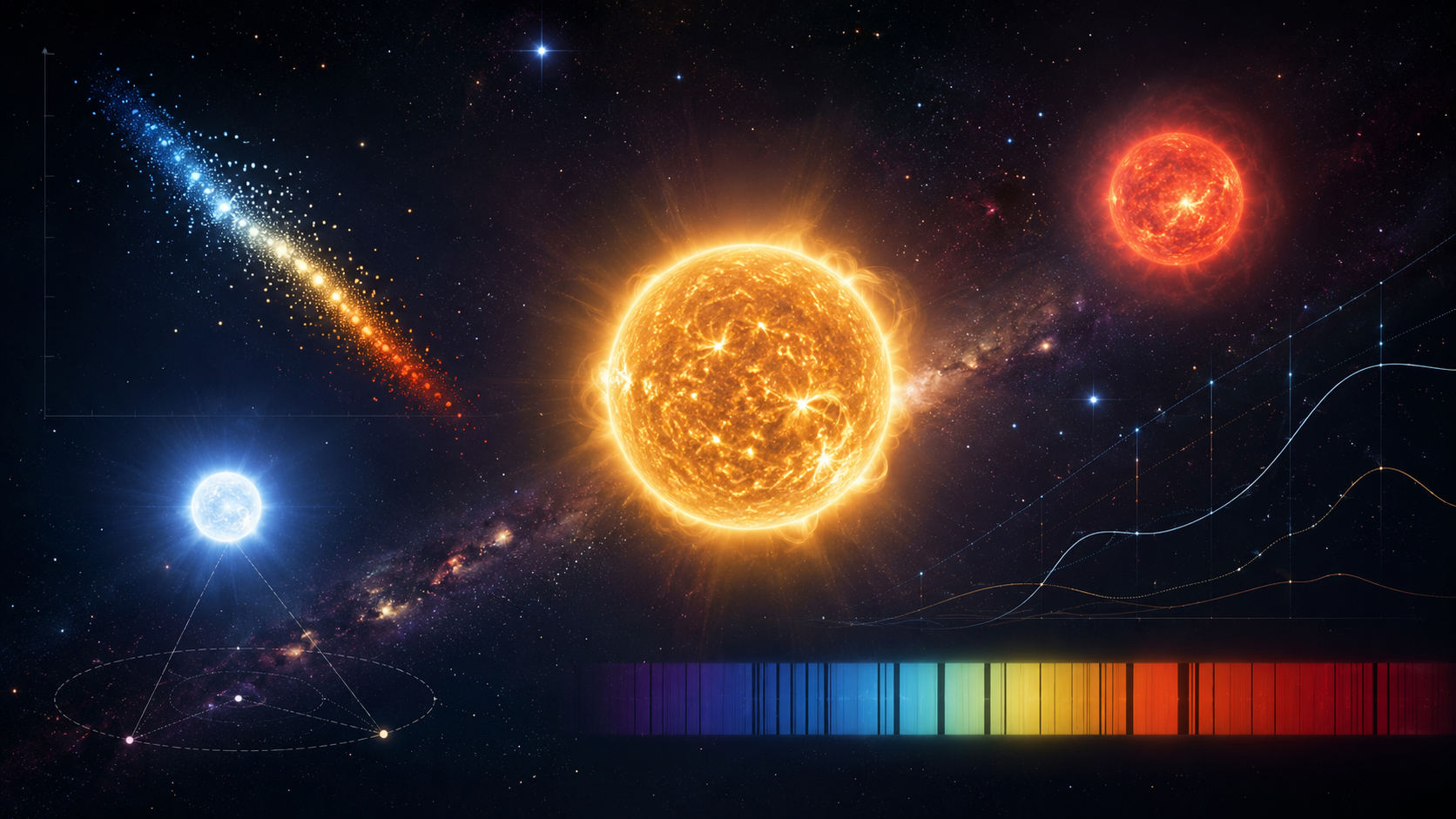
Stars, From Birth to Remnant Part 1: A First Look at the Sky

Stars: From Birth to Remnant, Part 1: A First Look at the Sky

Introduction

Humanity has never stopped looking up at the sky. Our ancestors, who made the first drawings on cave walls, took those shining points for gods of fire; later, as their thinking advanced a little further, they came to believe that the stars wrote our destinies. Even today, millions of people believe that their zodiac sign governs their mood. For a scientist, that is no longer a question of celestial mechanics, but of social psychology.

Yet whether you are an astrologer or an astrophysicist, one fact does not change: without the stars in the sky, we would not be here. Stars are the chemical factories of the universe. The oxygen we breathe, the iron in our blood, the gold in our phones—all were once produced in the core of a star. When we say, “We are stardust,” the first thing the naked eye notices is precisely color; and color directly reveals surface temperature. We are now going to build that bridge. Our aim is to develop that statement, together with all the physics behind it, step by step, without taking a single equation for granted.

This article is written for two readers at once. Someone reading the main text should be able to follow the story fluently without being buried in formulas; someone who ventures into the sections headed Derivation should see where every equation comes from, without a single step omitted. Often these two readers are the same person; it simply depends on the question they happen to be asking that day: sometimes, “How beautiful the stars are,” and sometimes, “But how do we know that?” The text must answer both.

What Is a Star?

Let us begin with the shortest possible definition, and then do justice to every word of it in the sections ahead.

Definition (Star):
A star is a sphere of plasma held together by its own gravity, in hydrostatic and thermal equilibrium, whose center has reached temperatures and pressures high enough to sustain long-term thermonuclear fusion.

Three phrases in this definition are critical; lose even one, and the object before us is no longer a “star.”

1. Equilibrium under its own gravity. Every layer of a star must support the weight above it. It does so through pressure that increases inward. The exact balance between inward-pulling gravity and the outward-acting pressure gradient is called hydrostatic equilibrium; in Part 2, we will derive this balance as a differential equation. For now, the verbal picture is enough: gravity says collapse, pressure refuses.

2. Sustainable thermonuclear fusion. If a sphere of gas is heating only by contraction and cannot convert hydrogen into helium in its core, we call it a brown dwarf, not a star. The hallmark of a true star is its ability to sustain, for billions of years, the core reaction

$$4\,^1\text{H} \longrightarrow \,^4\text{He} + 2e^+ + 2\nu_e + 2\gamma + Q$$

(and related reactions). Here $Q \approx 26{,}73\,\text{MeV}$ is the energy released; in Part 4, we will calculate where this number comes from using the mass defect.

3. The plasma state. Stellar matter is neither solid, liquid, nor neutral gas. The temperature is so high that electrons have been stripped from nuclei; the medium is a plasma made of electrically conductive, charged particles. This is not a trivial choice of terminology: it is precisely this ionized structure that determines a star’s opacity, energy transport, and magnetic behavior.

Three Parameters That Define a Star

Here is the surprising part: although the definition above looks complicated, the entire fate of a star can in practice be predicted from just three numbers.

• Mass ($M$): the dominant parameter. More than anything else, mass determines a star’s central temperature, which fusion reactions can operate, how long it will live, and how it will die. We will see the same principle again and again: where there is mass, there is destiny.

• Chemical composition: generally specified by the mass fractions $X$ (hydrogen), $Y$ (helium), and $Z$ (everything else). In astrophysics, every element other than hydrogen and helium is collectively classed as a “metal.” Tell a chemist that gold and oxygen are both “metals” and you will hear an objection, but in astrophysics that is the definition of $Z$.

• Age ($t$): tells us which stage of its life cycle the star has reached. Two stars of the same mass and composition can look entirely different at different ages.

Much of what follows answers this question: given $M$, composition, and $t$, how do all the properties we observe in a star emerge? First, however, we need to define what we mean by “observed properties” in measurable terms. No matter how elegant a theory may be, observation is where it is tested.

Light: The Only Thing That Reaches Us from a Star

We cannot travel to a star and insert a thermometer. Almost the only data we have is the light that reaches us from it. We must therefore begin by defining two fundamental quantities associated with light—how much energy, and from how far away—precisely.

Flux and Luminosity

Definition (Luminosity and flux):
A star’s luminosity (radiant power) $L$ is the total energy it emits in all directions per unit time; its unit is the watt. The flux $F$ measured by an observer is the energy received per unit area per unit time at the observer’s location; its unit is $\text{W\,m}^{-2}$.

$L$ is an intrinsic property of the star, independent of the observer; it is the star’s true power output. $F$ depends on where we stand. The relation connecting the two is a cornerstone of all observational astrophysics.

Example: Derivation (Inverse-square law)
Let us treat the star as a point source in empty space, with no matter around it. If the star emits energy equally in every direction (isotropic radiation), then the total energy it releases per unit time is $L$.

Imagine a sphere of radius $d$ centered on the star. If energy is neither created nor destroyed along the way, the total energy crossing the entire surface of this sphere per unit time must equal the energy emitted by the source:
$\oint_{\text{küre}} F\,\mathrm{d}A = L.$

By the assumption of isotropy, $F$ is the same at every point on the sphere and can be taken outside the integral. Because the surface area of a sphere of radius $d$ is $4\pi d^2$:

$F \cdot 4\pi d^2 = L \implies \boxed{F = \frac{L}{4\pi d^2}}$

Physical Interpretation:
Flux decreases with the square of distance because a fixed amount of energy is spread over a spherical surface whose area grows as $d$ as $d^2$ increases. Of two otherwise identical stars, one twice as distant appears four times dimmer. A star that looks faint in the sky may therefore be intrinsically weak or simply very far away; flux alone cannot distinguish between the two. Here lies astrophysics’ oldest nuisance: distance.

The assumptions of “isotropic” emission and “no intervening matter” are not innocuous. Real stars are slightly flattened by rotation and radiate differently at their poles and equators; interstellar dust also absorbs light (interstellar extinction). We will introduce these corrections one by one later. For now, we are constructing the basic framework.

The Magnitude System

Astronomy expresses brightness on a scale that is peculiar, yet deeply rooted in history. In the second century BCE, Hipparchus classified the brightest stars as “first magnitude” and those barely visible to the naked eye as “sixth magnitude.” In the nineteenth century, Norman Pogson quantified this old classification and found that the five steps between first and sixth magnitude corresponded to a flux ratio of approximately 100. He turned this into an exact definition.

Definition (Pogson relation):
For two sources with apparent magnitudes $m_1,\,m_2$ and fluxes $F_1,\,F_2$, the relation
$m_1 - m_2 = -2{,}5\log_{10}\!\left(\frac{F_1}{F_2}\right)$
serves as the definition.

[!example] Derivation (Where does the coefficient −2.5 come from?)
We require two conditions. First, the scale must be logarithmic: a fixed flux ratio must correspond to a fixed magnitude difference. This forces a relation of the form $m_1 - m_2 = C\log_{10}(F_1/F_2)$; all that remains is to determine the constant $C$.

The second condition is the historical fact measured by Pogson: a magnitude difference of exactly 5 must correspond to a flux ratio of exactly 100. By the old convention, moreover, the brighter star has the smaller magnitude, so $C$ must be negative. Let $F_1/F_2 = 1/100$ when $m_1 - m_2 = +5$:
$5 = C\log_{10}\!\left(\tfrac{1}{100}\right) = C \cdot (-2) \implies C = -\frac{5}{2} = -2{,}5.$

The coefficient is therefore not arbitrary; it follows directly from the rule “5 magnitudes = a factor of 100.”

Interlude:
The magnitude scale has two irritating features, both inherited from history. First, a smaller number means a brighter object. The Sun’s apparent magnitude is $-26{,}7$, while Sirius has $-1{,}5$. Second, the scale is logarithmic, so a “difference of 1” does not mean the same additive difference in brightness everywhere; it always means the same ratio ($\approx 2{,}512$). Modern astronomers use this scale not because they love it, but because they must remain compatible with 2,000 years of data.

Absolute Magnitude and the Distance Modulus

Apparent magnitude $m$ measures flux, so it is entangled with distance. To express the star’s intrinsic luminosity in the language of magnitudes, we need a trick that amounts to moving every star to the same distance.

Definition (Absolute magnitude):
A star’s absolute magnitude $M$ is the apparent magnitude it would have if it were located at a distance of exactly 10 pc.

Derivation (Distance modulus):
Let us “observe” the same star twice: once at its true distance $d$ (apparent magnitude $m$, flux $F$), and once at 10 pc (apparent magnitude $M$ by definition, flux $F_{10}$). Apply the Pogson relation to these two cases:

$m - M = -2{,}5\log_{10}\!\left(\frac{F}{F_{10}}\right).$

The star’s luminosity $L$ is the same in both cases; only the distance has changed. From the inverse-square law,

$F = \frac{L}{4\pi d^2}, \quad F_{10} = \frac{L}{4\pi(10\,\text{pc})^2} \implies \frac{F}{F_{10}} = \left(\frac{10\,\text{pc}}{d}\right)^2.$

Substituting:

$m - M = -2{,}5\log_{10}\!\left[\left(\frac{10\,\text{pc}}{d}\right)^2\right] = -5\log_{10}\!\left(\frac{10\,\text{pc}}{d}\right).$

Invert the fraction inside the logarithm and absorb the sign:

$\boxed{m - M = 5\log_{10}\!\left(\frac{d}{10\,\text{pc}}\right) = 5\log_{10}\!\left(\frac{d}{\text{pc}}\right) - 5}$

The quantity $m - M$ on the left-hand side is called the distance modulus.

Physical Interpretation:
The distance modulus converts the difference between “how bright it looks” and “how luminous it really is” directly into a distance. We measure $m$ observationally. If $M$ can be determined independently—and in later parts we will do exactly that using methods such as Cepheid variables and main-sequence fitting—then $d$ is the only remaining unknown, and the distance can be solved for. The entire cosmic distance ladder is built upon this equation.

The First Rung of the Distance Ladder: Trigonometric Parallax

The distance modulus is useful, but knowing $M$ often already requires knowing the star’s distance—a classic circular problem. The first, most direct method with the fewest assumptions to break this circle is trigonometric parallax: pure geometry.

Derivation (Parallax and the parsec):
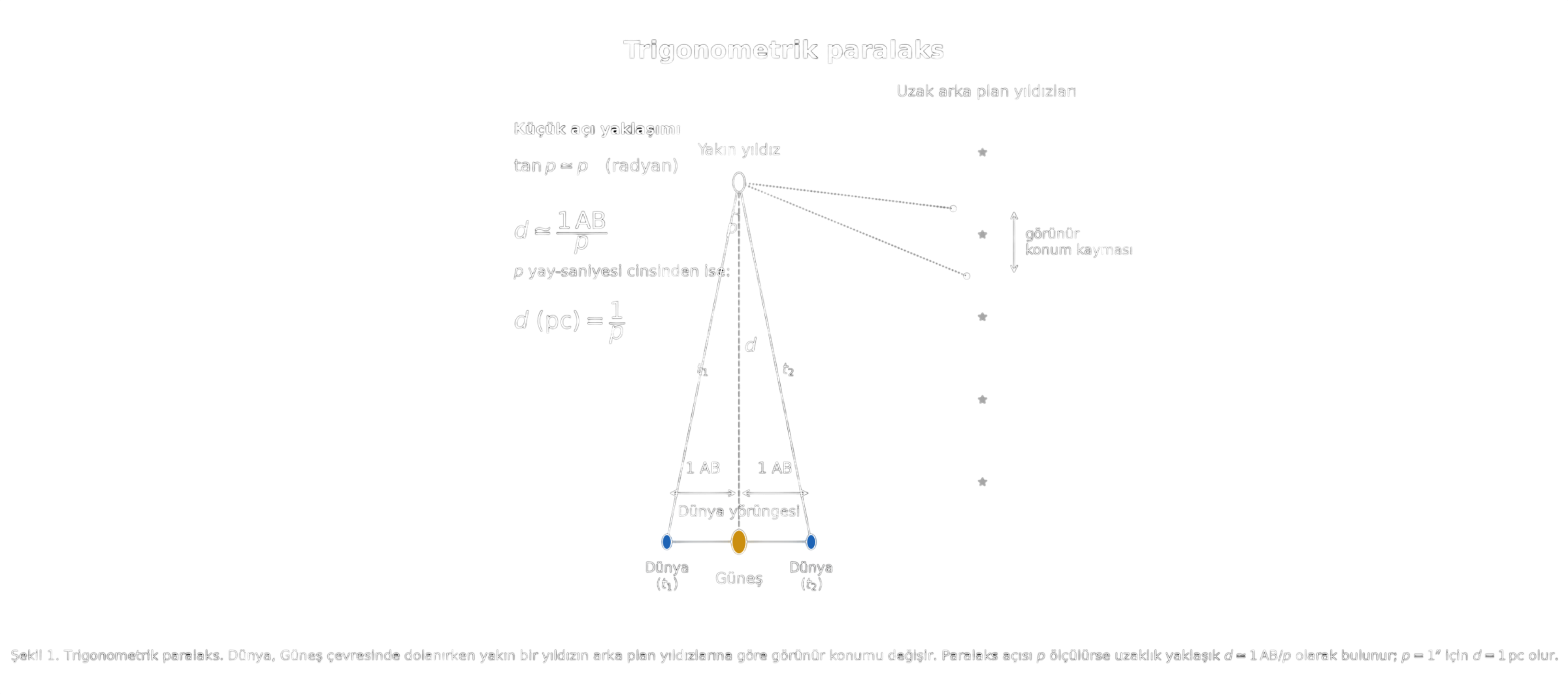
Earth orbits the Sun on an orbit with a radius of 1 astronomical unit (1 AU). Observations six months apart place Earth at opposite ends of its orbit, giving a baseline of 2 AU. Owing to this motion, a nearby star appears to trace a small ellipse relative to very distant background stars.

The parallax angle $p$ is defined as half this apparent displacement: the angle subtended by 1 AU between Earth and the Sun as viewed from the star. The star, Sun, and Earth form a right triangle; its perpendicular sides are 1 AU and $d$, with angle $p$ at the star:

$\tan p = \frac{1\,\text{AB}}{d}.$

Stars are so distant that $p$ is always very small (less than $1''$ even for the nearest star). Under the small-angle approximation, $\tan p \approx p$ (in radians):

$d \approx \frac{1\,\text{AB}}{p}.$

Let us measure $p$ in arcseconds ($''$). Since $1'' = 1/206265$ radians, it is natural to absorb this unit into the equation by defining a new unit of distance:

$1\,\text{parsek} \equiv \frac{1\,\text{AB}}{1''\,[\text{radyan}]} = 206265\,\text{AB} \approx 3{,}086 \times 10^{16}\,\text{m} \approx 3{,}26\,\text{ışıkyılı}.$

The name “parsec” itself comes from parallax of one arcsecond. In this unit, the relation takes its simplest form:

$\boxed{d\,[\text{pc}] = \frac{1}{p\,['']}}$

Physical Interpretation:
The parsec is not a unit chosen by human whim; it is the scale that emerges naturally from the parallax equation. By measuring these angles at the level of microarcseconds, the Gaia satellite has determined the distances of more than a billion stars from this single equation, without making any astrophysical assumptions. Geometry is the first and firmest rung of the cosmic distance ladder.

Interlude:
Parallax has a brutally honest side: as the angle you measure becomes smaller—that is, as the star grows more distant—the uncertainty increases mercilessly. Trigonometric parallax is therefore reliable only for “nearby” stars: a few hundred parsecs before Gaia, a few thousand parsecs with Gaia. For the far side of the Galaxy or for other galaxies, we must climb to the higher rungs of the ladder. We will construct those rungs one by one in later parts, but every one of them ultimately rests on this pure triangle.

Effective Temperature and Blackbody Radiation

So far, we have learned to measure how much energy reaches us from a star (flux, luminosity, magnitude) and how far away it is (parallax). We have not yet addressed the star’s color or temperature. Color is precisely the first thing the naked eye notices in a star, and it directly reveals the surface temperature. Let us now build that bridge.

We cannot insert a thermometer into a star; all we can collect is its light. Fortunately, stellar radiation is approximately blackbody radiation, and the spectrum of a blackbody depends on only one parameter: its temperature. The goal of this section is to derive the two fundamental blackbody laws—Stefan–Boltzmann and Wien—from the Planck distribution, step by step, and from there arrive at the operational definition of “stellar temperature,” the effective temperature $T_\text{eff}$.

The Blackbody Concept

An object that completely absorbs all radiation incident upon it, at every wavelength, is called a blackbody. The name is misleading: a blackbody in thermal equilibrium also emits radiation and may in fact be extremely bright; “black” refers only to its perfect absorptivity. Kirchhoff’s profound 1859 result was this: the radiation emitted by a body in thermal equilibrium depends only on its temperature, independently of its material, geometry, or date of manufacture. This universal radiation is blackbody radiation.

Interlude:
A star is not, of course, an ideal blackbody. In its upper atmosphere, particular atoms selectively absorb photons at particular frequencies and carve lines into the stellar spectrum. But these line systems are small notches superimposed on the continuum; in terms of integrated flux, the continuous, nearly blackbody spectrum dominates. The optically thick and slowly varying temperature structure of a stellar photosphere largely satisfies the condition of “local thermodynamic equilibrium” (LTE), which is enough for Kirchhoff’s theorem to apply.

The Planck Distribution

Planck’s universal radiation law, discovered in 1900, is:

Definition (Planck function):
The specific intensity emitted by a blackbody at temperature $T$, per unit area, per unit solid angle, and per unit frequency interval, is

$B_\nu(T) = \frac{2h\nu^3}{c^2} \cdot \frac{1}{\exp(h\nu/kT) - 1}.$

Its unit is $\text{W\,m}^{-2}\text{\,Hz}^{-1}\text{\,sr}^{-1}$.

The Planck function has three regimes:

• Low frequency (Rayleigh–Jeans regime): when $h\nu \ll kT$, expand the exponential: $\exp(h\nu/kT) - 1 \approx h\nu/kT$. The result is

$$B_\nu \approx \frac{2\nu^2 kT}{c^2}.$$

Classical physics (Maxwell’s equations plus equipartition) gave the same result, but extending it to all frequencies made the total energy diverge (the “ultraviolet catastrophe”). Planck’s exponential cutoff is precisely what averts that catastrophe.

• High frequency (Wien tail): when $h\nu \gg kT$, $\exp(h\nu/kT) - 1 \approx \exp(h\nu/kT)$, and

$$B_\nu \approx \frac{2h\nu^3}{c^2}\exp(-h\nu/kT).$$

The flux falls exponentially; there is very little thermal energy available to produce photons of such high energy.

• Peak: between these two regimes, $B_\nu$ reaches a peak; the peak frequency is directly proportional to temperature (Wien’s law, which we will derive shortly).

The Stefan–Boltzmann Law: $F = \sigma T^4$

To find the total energy output, the Planck distribution must be integrated over all frequencies.

Derivation (Stefan–Boltzmann law):
The total outward flux per unit area is found by integrating the Planck intensity over frequency and over solid angle across the outward hemisphere (weighted by $\cos\theta$). The angular integral $\int\cos\theta\,\mathrm{d}\Omega$ over a hemisphere equals $\pi$ (Lambert’s cosine law). This leaves:

$F = \pi\int_0^\infty B_\nu(T)\,\mathrm{d}\nu = \frac{2\pi h}{c^2}\int_0^\infty \frac{\nu^3}{e^{h\nu/kT}-1}\,\mathrm{d}\nu.$

Introduce the dimensionless variable $x = h\nu/kT$, so that $\mathrm{d}\nu = (kT/h)\,\mathrm{d}x$.

$\int_0^\infty \frac{\nu^3}{e^{h\nu/kT}-1}\,\mathrm{d}\nu = \left(\frac{kT}{h}\right)^4 \int_0^\infty \frac{x^3}{e^x - 1}\,\mathrm{d}x.$

The final integral is a standard identity. Expanding $1/(e^x - 1) = \sum_{n=1}^\infty e^{-nx}$, integrating term by term, and using $\int_0^\infty x^3 e^{-nx}\,\mathrm{d}x = 6/n^4$ gives:

$\int_0^\infty \frac{x^3}{e^x - 1}\,\mathrm{d}x = 6\sum_{n=1}^\infty \frac{1}{n^4} = 6\zeta(4) = 6 \cdot \frac{\pi^4}{90} = \frac{\pi^4}{15}.$

($\zeta(s) = \sum_n 1/n^s$ is the Riemann zeta function; $\zeta(4) = \pi^4/90$.) Substituting back:

$F = \frac{2\pi h}{c^2} \cdot \left(\frac{kT}{h}\right)^4 \cdot \frac{\pi^4}{15} = \frac{2\pi^5 k^4}{15\,c^2 h^3}\,T^4 \equiv \sigma T^4.$

The Stefan–Boltzmann constant is

$$\sigma = \frac{2\pi^5 k^4}{15\,c^2 h^3} \approx 5{,}67 \times 10^{-8}\,\text{W\,m}^{-2}\text{\,K}^{-4}.$$

and the total flux per unit area is

$$\boxed{F = \sigma T^4}$$

Physical Interpretation:
The dependence on the fourth power of temperature is extraordinary: double the temperature and the energy output rises by a factor of 16. This is the mathematical origin of the enormous luminosity difference between hot and cool stars.

Wien’s Displacement Law:

How does the peak of the Planck distribution—the peak that determines the star’s “color”—depend on temperature?

Derivation (Wien’s law):
To find the maximum of $B_\nu$ with respect to $\nu$, set the derivative to zero. Using the dimensionless variable $x = h\nu/kT$:

$B_\nu \propto \frac{x^3}{e^x - 1}.$

The derivative is

$\frac{\mathrm{d}}{\mathrm{d}x}\frac{x^3}{e^x - 1} = \frac{3x^2(e^x - 1) - x^3 e^x}{(e^x - 1)^2}.$

The numerator must vanish ($x = 0$ is not a peak because it also makes the denominator vanish):

$3x^2(e^x - 1) = x^3 e^x \implies 3(1 - e^{-x}) = x.$

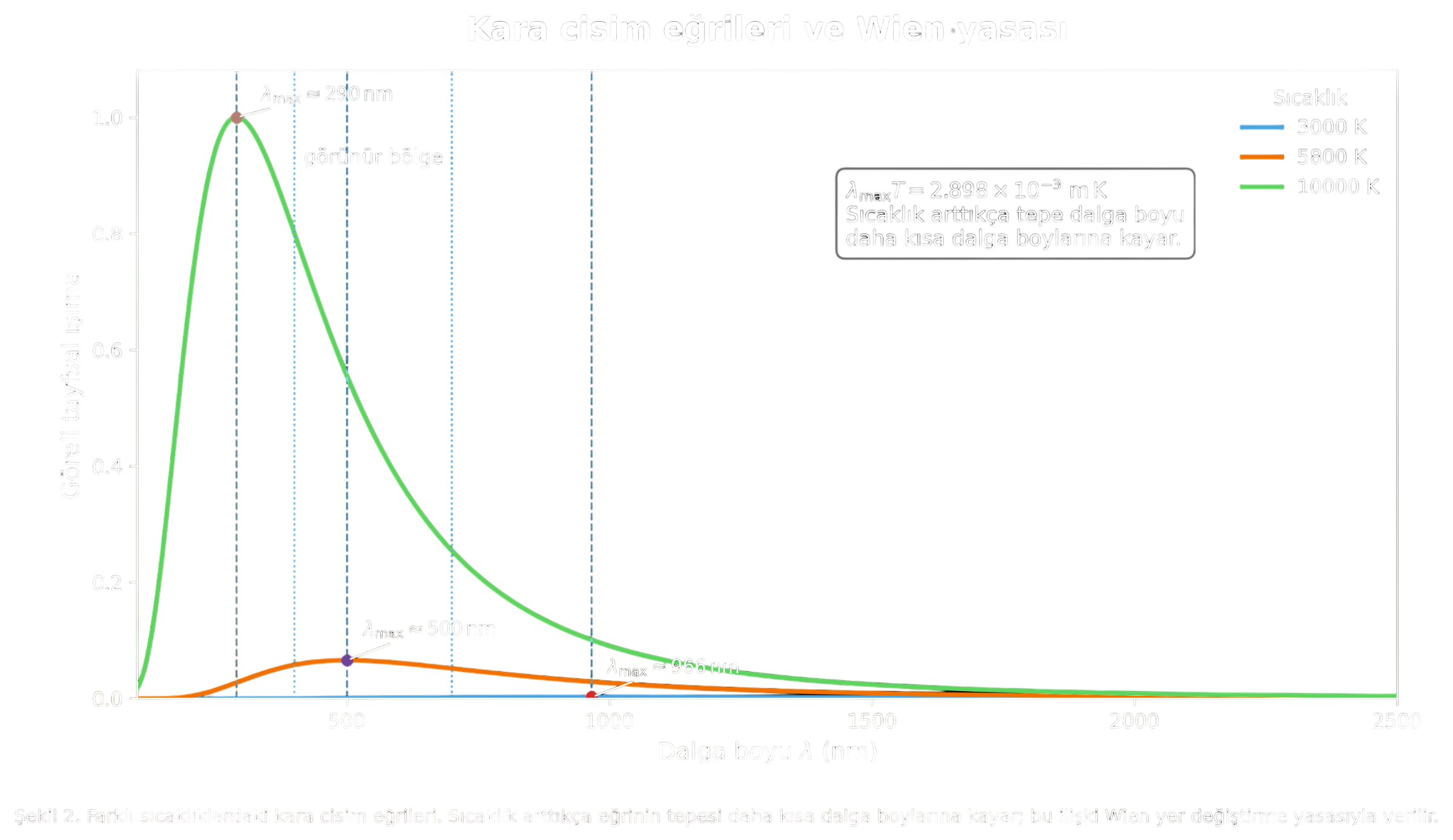
This is a transcendental equation with no closed-form solution. Its numerical solution is $x \approx 2{,}821$. From the definition $x = h\nu_\text{max}/(kT)$:

$\boxed{\frac{\nu_\text{max}}{T} = \frac{2{,}821\,k}{h} \approx 5{,}88 \times 10^{10}\,\text{Hz\,K}^{-1}}$

For the wavelength formulation, the peak of $B_\lambda$ is obtained from a separate transcendental equation ($x \approx 4{,}965$):

$$\lambda_\text{max}\,T \approx 2{,}898 \times 10^{-3}\,\text{m\,K}.$$

Example:
For the Sun, $T_\odot \approx 5778\,\text{K}$ gives $\lambda_\text{max} \approx 501\,\text{nm}$, in the yellow-green region of the visible spectrum. For an M-class dwarf ($T \approx 3500\,\text{K}$), $\lambda_\text{max} \approx 830\,\text{nm}$ (near-infrared). For an O star ($T \approx 35.000\,\text{K}$), $\lambda_\text{max} \approx 83\,\text{nm}$ (far ultraviolet); it appears “blue-white” in visible light.

Physical Interpretation:
Wien’s law lets us read a star’s temperature by looking at the sky. A blue star is hot (short $\lambda_\text{max}$); a red star is cool.

Effective Temperature

(Effective temperature):
A star’s effective temperature $T_\text{eff}$ is the temperature of an ideal blackbody with the same radius and total luminosity as the star. Operationally:

$\boxed{L = 4\pi R^2 \sigma T_\text{eff}^4}$

Physical Interpretation:
$T_\text{eff}$ is not literally “the star’s surface temperature”; there may be no material anywhere in the star at exactly this value. A stellar atmosphere typically has a temperature close to $\tau \approx 2/3$ at the point where the optical depth is of order unity ($T_\text{eff}$).

Example:
For the Sun, $L_\odot = 3{,}828 \times 10^{26}\,\text{W}$ and $R_\odot = 6{,}96 \times 10^8\,\text{m}$. From Stefan–Boltzmann:

$T_{\text{eff},\odot}^4 = \frac{L_\odot}{4\pi R_\odot^2 \sigma} \implies T_{\text{eff},\odot} \approx 5778\,\text{K}.$

Color, Color Index, and Bolometric Correction

Filter Systems

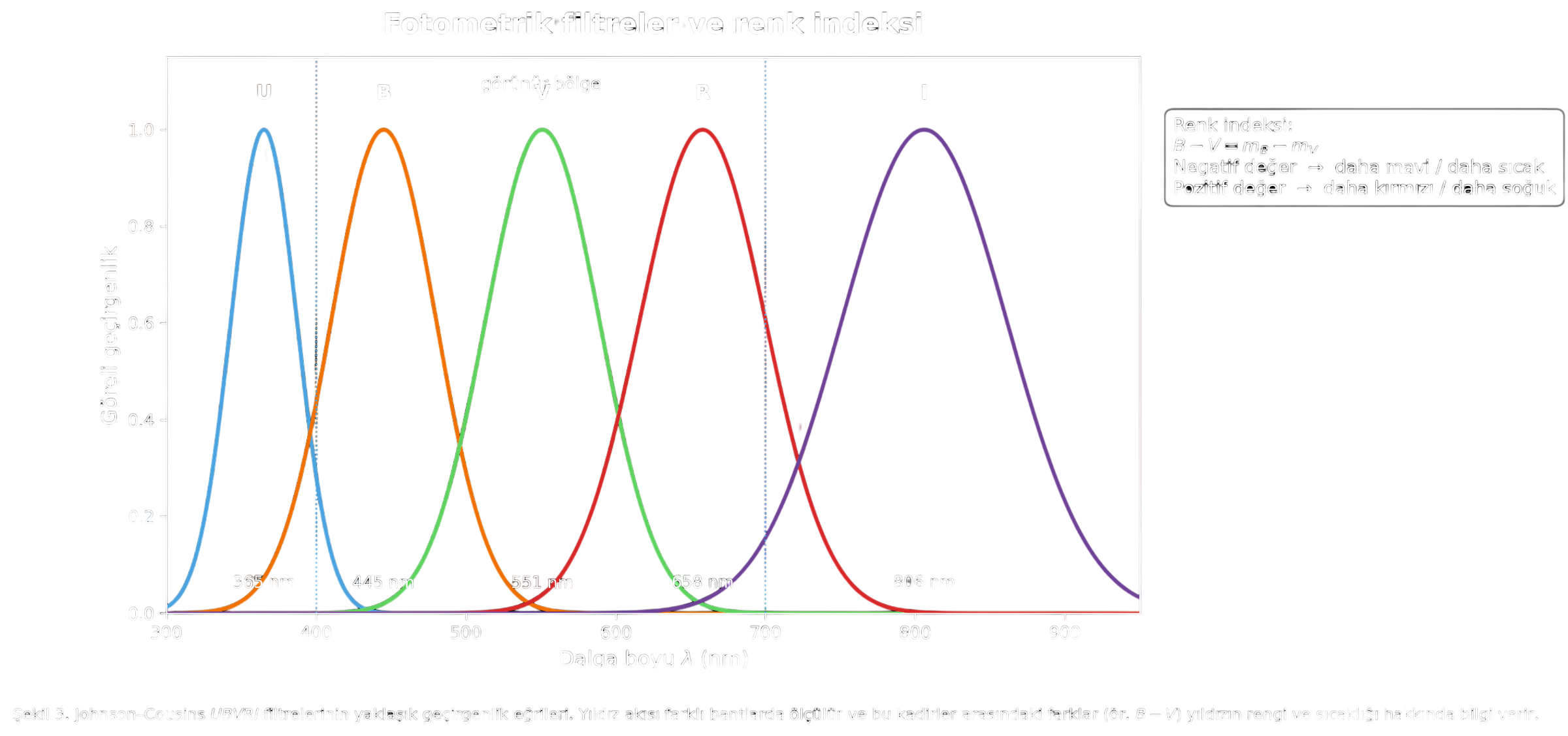
Observers generally measure stellar flux through several standard filters. The most widely used classical system is Johnson–Cousins $UBVRI$:

• $U$ (ultraviolet), centered at $\sim 365\,\text{nm}$
• $B$ (blue), $\sim 445\,\text{nm}$
• $V$ (visual/yellow-green), $\sim 551\,\text{nm}$
• $R$ (red), $\sim 658\,\text{nm}$
• $I$ (near-infrared), $\sim 806\,\text{nm}$

Modern surveys (SDSS, Pan-STARRS, Gaia) use different filter systems, but the principle is the same.

Color Index

Definition (Color index):
The difference between apparent magnitudes in two bands is called a color index. The most commonly used is $B - V$:

$(B - V) \equiv m_B - m_V.$

By convention, Vega ($\alpha$ Lyr) is the zero reference for every color index. Approximate values for main-sequence stars are:

Class	$B-V$	$T$ (K)
O5	$\approx -0{,}33$	$\sim 35.000$
A0	$= 0{,}00$	$\sim 10.000$
G2 (Sun)	$\approx 0{,}66$	$\sim 5800$
M0	$\approx 1{,}40$	$\sim 3700$

Physical Interpretation:
The color index is independent of the individual distance: both $B$ and $V$ weaken by the same factor of $1/d^2$, so their difference remains unchanged. Color is therefore an intrinsic property of the star; its distance need not be known.

Interstellar Reddening

Dust between us and the star absorbs short wavelengths more strongly than long wavelengths. This interstellar reddening increases the measured $B - V$. We work with the “intrinsic” color,

$$(B - V)_0 = (B - V)_\text{gözlem} - E(B - V)$$

where $E(B - V)$ is the color excess.

Bolometric Correction

Definition (Bolometric correction):
The difference between a star’s bolometric magnitude $M_\text{bol}$ and its $V$-band absolute magnitude $M_V$ is called the bolometric correction:

$\text{BC} \equiv M_\text{bol} - M_V.$

Taking the Sun as the standard reference, the connection between $M_\text{bol}$ and $L$ is

$$M_\text{bol} - M_{\text{bol},\odot} = -2{,}5\log_{10}\!\left(\frac{L}{L_\odot}\right).$$

By an IAU resolution in 2015, $M_{\text{bol},\odot} = +4{,}74$ was fixed.

Interlude:
It is important to state the band to which the bolometric correction is applied. The $V$ band is standard in the classical literature; modern work often favors the infrared ($K$ or $J$ band).

Spectra and the Origin of Spectral Lines

Kirchhoff’s Three Laws

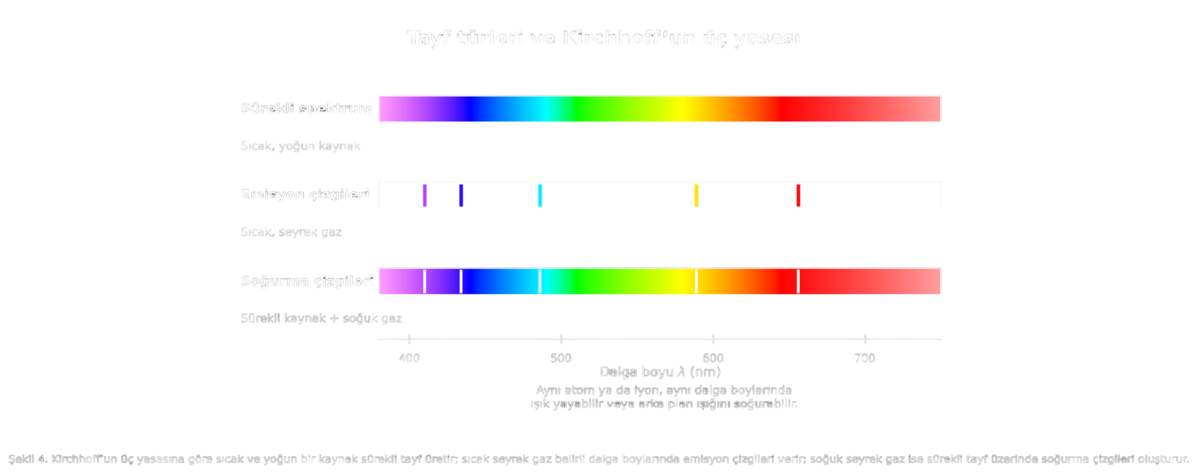
1. A hot, optically thick source emits a continuous spectrum.
2. A hot, optically thin gas produces a line emission spectrum.
3. A cooler, optically thin gas in front of a continuous source produces absorption lines.

A star corresponds to the third case: the inner regions produce a continuous spectrum, while the cooler atmosphere carves out lines before the radiation escapes.

The Atomic Origin of Lines

A bound electron in an atom can occupy only discrete energy levels. When a photon is absorbed, the electron jumps from a lower level to a higher one:

$$h\nu_{nm} = E_n - E_m.$$

Every element—and every ion—has its own characteristic pattern of energy levels; the wavelength pattern of its absorption lines is that atom’s “fingerprint.”

Three Dependencies of Line Strength

1. The abundance of that element in the atmosphere. More atoms, a stronger line.
2. The fraction of those atoms in the ionization stage that produces the line.
3. The probability that an ion occupies the lower electronic level responsible for the line. Boltzmann excitation: $n_m/n_0 \propto g_m \exp(-E_m/kT)$.

Physical Interpretation:
The competition between the second and third factors explains why spectral lines reach maximum strength over particular temperature ranges. The classic example is the hydrogen Balmer series. Balmer lines peak at approximately $T \approx 10.000\,\text{K}$ (in A-class stars); that is why Balmer lines are strongest in A-class stars.

Spectral Classes: The Harvard and MK Systems

The Harvard Sequence: OBAFGKM

Definition (Harvard spectral classes):
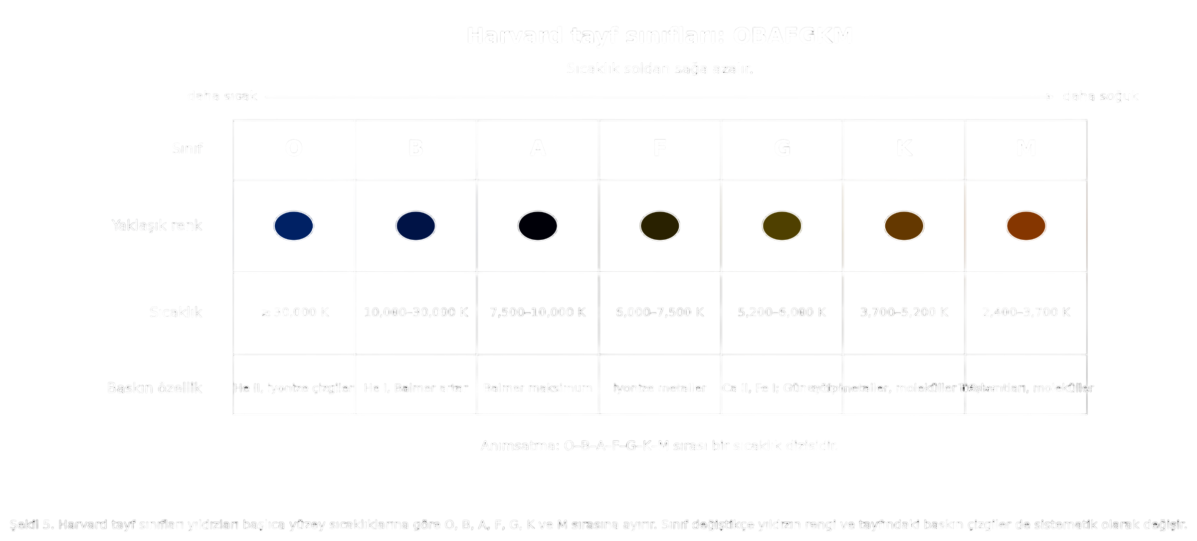
Stars are grouped by surface temperature in the following descending order:

$O \to B \to A \to F \to G \to K \to M$

and each class is divided into subclasses from 0 to 9 (e.g., G2 = the Sun).

The signature of each class is:

• O ($\gtrsim 30.000\,\text{K}$): lines of ionized helium (He II), ionized nitrogen, oxygen, and silicon.
• B (10.000–30.000 K): neutral helium (He I) dominates; hydrogen Balmer lines strengthen.
• A (7500–10.000 K): Balmer lines at their maximum strength; ionized-metal lines begin to appear.
• F (6000–7500 K): Balmer lines weaken; ionized metals (Ca II) strengthen.
• G (5200–6000 K, the Sun): neutral metals (Ca I, Fe I) and ionized Ca (the H and K lines) are very strong.
• K (3700–5200 K): neutral-metal lines dominate; the first molecular bands (TiO) appear.
• M (2400–3700 K): TiO molecular bands dominate.

Interlude:
The mnemonic “Oh Be A Fine Girl/Guy, Kiss Me” helps with the OBAFGKM sequence. Cannon and her predecessors initially used an alphabetical sequence (A, B, C, …); after the classes were reordered by temperature, gaps remained in the lettering.

Morgan–Keenan Luminosity Classes

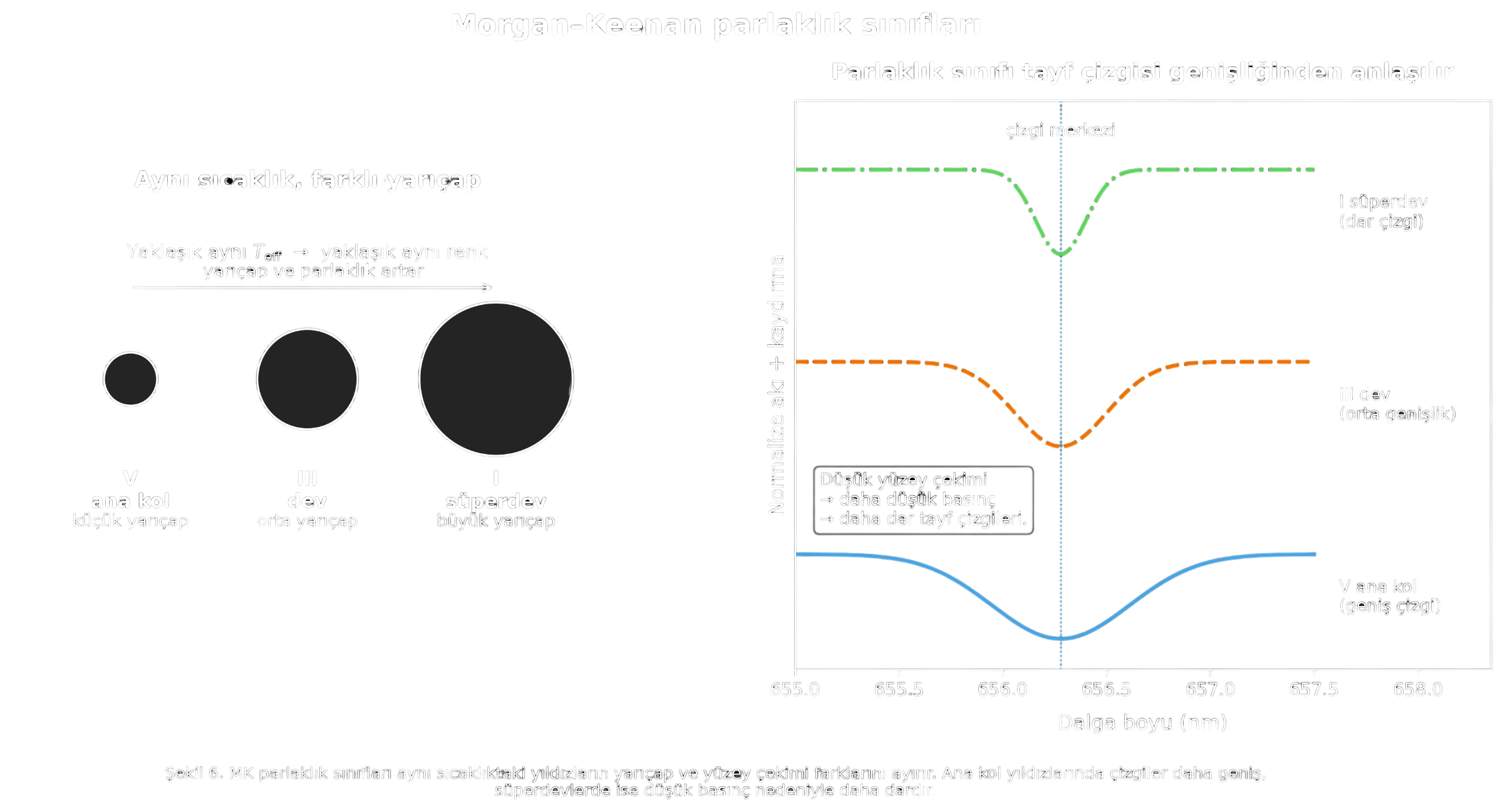
In 1943, Morgan and Keenan added luminosity classes, denoted by Roman numerals:

Class	Description
Ia, Ib	luminous/faint supergiant
II	bright giant
III	giant
IV	subgiant
V	main sequence (dwarf); the Sun is G2V
VI	subdwarf
VII	white dwarf

The spectral diagnostic of luminosity class is line width: the chain is “line width → atmospheric pressure → surface gravity → stellar radius.”

Complete Classification Examples

Example — Full classifications of several famous stars:

• Sun: G2V
• Sirius A ($\alpha$ CMa A): A1V
• Vega ($\alpha$ Lyr): A0V (color standard)
• Betelgeuse ($\alpha$ Ori): M1-2 Ia-ab (red supergiant)
• Rigel ($\beta$ Ori): B8 Ia (blue supergiant)
• Aldebaran ($\alpha$ Tau): K5 III (red giant)
• Procyon B: DF (a white dwarf with an F-type spectrum)

The Hertzsprung–Russell Diagram

Historical Background

In 1905, Ejnar Hertzsprung recognized a correlation between color and absolute luminosity. In 1913, Henry Norris Russell independently showed that a similar pattern appeared in the plane of spectral class versus absolute magnitude. Combining the two lines of work made the HR diagram an enduring tool.

Observational and Theoretical HR Diagrams

Observational HR (color–magnitude diagram, CMD). The horizontal axis is color index (usually $B - V$), and the vertical axis is absolute magnitude $M_V$.

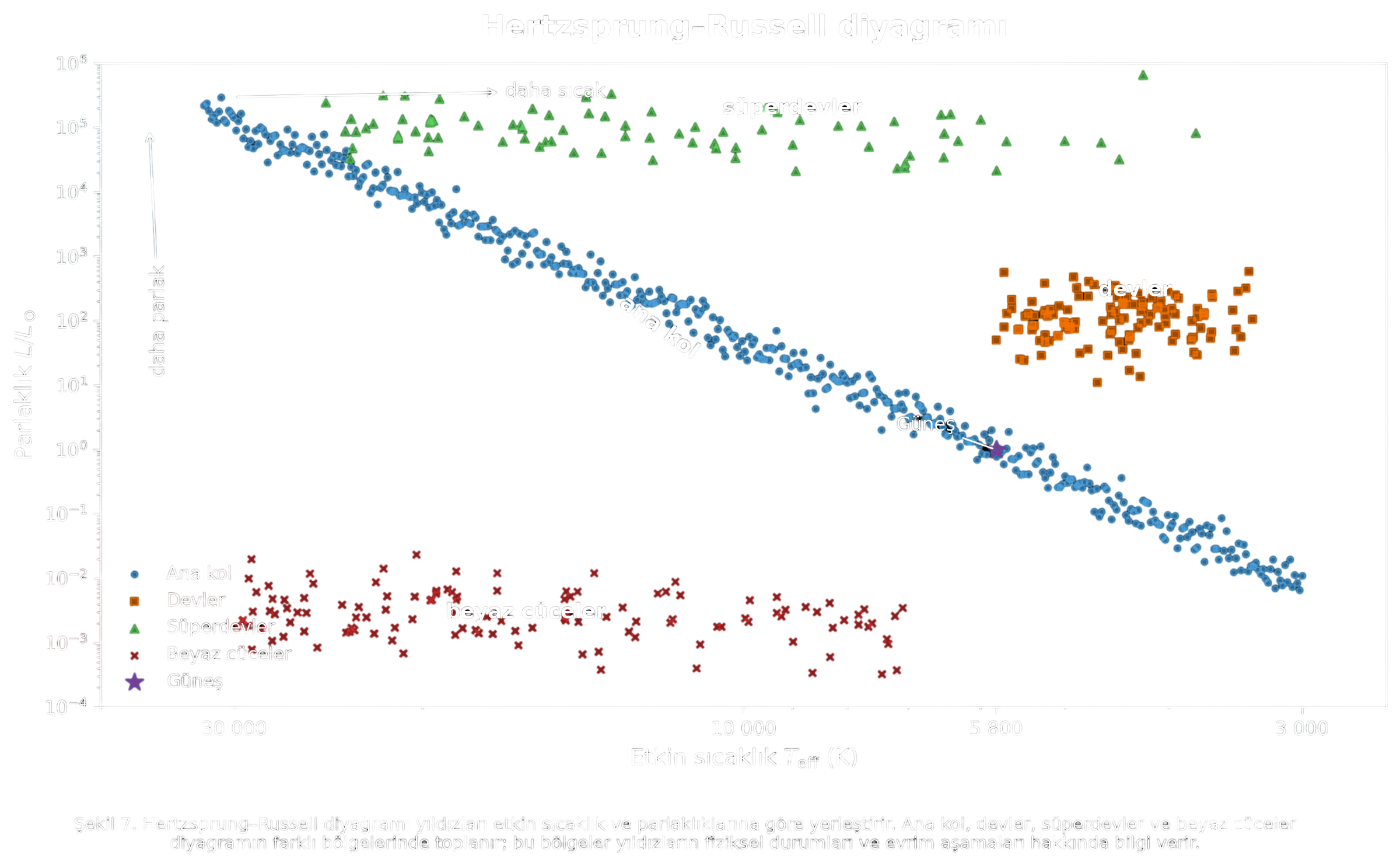
Theoretical HR. The horizontal axis is $\log T_\text{eff}$, running in the decreasing direction (hotter stars on the left), and the vertical axis is $\log(L/L_\odot)$.

The Geography of the HR Diagram

• Main sequence. A broad diagonal running from upper left to lower right. The great majority of stars lie here, from $\sim 100\,M_\odot$ O stars at the top to $\sim 0{,}08\,M_\odot$ M dwarfs at the bottom.

• Giant branch and supergiants. In the upper-middle region of the diagram: the red giant branch (RGB), asymptotic giant branch (AGB), and horizontal branch. Supergiants ($\gtrsim 10\,M_\odot$) stretch horizontally across the topmost band.

• White dwarfs. In the lower-left corner of the diagram: high $T_\text{eff}$ and low $L$. As they cool, they move downward and to the right.

Between the main sequence and the giant branch lies a sparsely populated region called the “Hertzsprung gap.” Stars are rarely caught there because they cross it on the short thermal timescale.

8.4 Why the HR Diagram Is So Valuable

Physical Interpretation:
Which regions are populated and which remain empty in a stellar population is dictated directly by stellar evolution. In observations of a cluster, its age can be inferred from the point where its isochrone leaves the main sequence—the turnoff. The composition and star-formation history of the stellar population in a distant galaxy can be read from the geography of its HR diagram.

How Stellar Mass and Radius Are Measured

Binary-Star Systems: The Gold Standard for Mass

Derivation (Total mass from Kepler’s third law):
Let two stars orbit their common center of mass on elliptical trajectories. Kepler’s third law, in its Newtonian form, is

$\frac{a^3}{P^2} = \frac{G\,M_\text{tot}}{4\pi^2}.$

In astronomical units:

$\boxed{M_\text{tot}\,[M_\odot] = \frac{a^3\,[\text{AB}]}{P^2\,[\text{yıl}]}}$

For the individual masses, the definition of the center of mass gives

$$M_1 a_1 = M_2 a_2 \implies \frac{M_1}{M_2} = \frac{a_2}{a_1}.$$

Types of Binary Systems

• Visual binary. The two stars can be resolved directly with a telescope.
• Spectroscopic binary. Radial velocities are measured from Doppler shifts in their spectra. The velocity ratio is $v_1/v_2 = M_2/M_1$.
• Eclipsing binary. The stars eclipse one another; the light curve gives the stellar radii directly. Detached eclipsing binaries (DEBs) yield accuracies better than one percent.
• Astrometric binary. An unseen companion is detected through the star’s positional wobble on the sky (Gaia).

Direct Measurement of Stellar Radius

• From the duration of an eclipsing-binary light curve. $R_1$ and $R_2$ are solved for directly. This is the most precise method.
• Interferometry. The angular diameter $\theta$ is measured; combining it with distance $d$ gives $R = d\theta/2$.
• Spectrum + Stefan–Boltzmann. $L = 4\pi R^2 \sigma T_\text{eff}^4$ gives $R$ directly.

In the modern era, asteroseismology is advancing rapidly: stellar radius, density profile, and age are inferred from the frequencies of oscillation modes (Kepler, TESS).

Interlude:
The oldest piece of knowledge here—Kepler’s seventeenth-century law—remains the gold standard for measuring mass. Binary measurements anchor the models to reality.

[!abstract] Next Part
This brings Part 1 to a close: we have seen how all the fundamental quantities that can be measured for a star—flux, luminosity, absolute magnitude, distance, temperature, color, spectral class, mass, and radius—are obtained through independent methods.

Now we turn to the star’s internal physics. In Part 2, we will lay out the equation of mechanical balance (hydrostatic equilibrium), the three sources of pressure (ideal gas, radiation, and the degenerate electron gas), ionization equilibrium (a complete derivation of the Saha equation), the virial theorem, and the characteristic timescales. Once energy transport is added in Part 3, we will have the four fundamental equations of stellar structure; then, beginning with nuclear reactions, we will follow the star from birth to remnant.