Semiconductor Physics Series Part 3: Introduction to the Quantum Theory of Solids

Energy Bands and the Kronig–Penney Model

Introduction

From the preceding article, we know that an isolated atom has discrete energy levels, as required by the Pauli exclusion principle. When determining the electrical properties of a semiconductor containing approximately $10^{21}$ atoms, however, the cumulative interaction of those discrete levels must also be considered. This leads us to energy bands. Energy-band theory is a fundamental principle of semiconductor-material physics and explains differences in the electrical properties of metals, insulators, and semiconductors. Here, we will first discuss the allowed and forbidden energy bands in a single-crystal solid qualitatively, then treat them mathematically using the wave equation.

Formation of Energy Bands

Energy-band formation is a natural many-electron consequence of the physical reality described by the Pauli exclusion principle. First consider hydrogen. Figure 1(a) shows its radial probability distribution. When two hydrogen atoms approach one another, their electron probability distributions overlap, as in (b). The perturbation caused by this interaction splits the energy levels because two electrons with the same quantum numbers cannot occupy the same atom. This splitting is shown in (c).

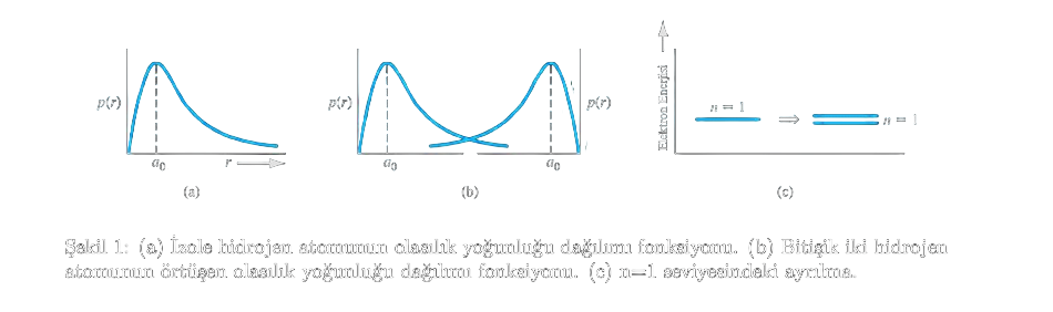
Many-electron systems likewise undergo this splitting at the equilibrium interatomic separation. The Pauli exclusion principle, however, tells us that bringing atoms together to form a system such as a crystal does not change the total number of quantum states. As the atoms approach, their discrete energy levels therefore split in different ways, forming bands that keep every electron in a distinct quantum state. Figure 2 schematically shows this splitting for multiple electrons. As interatomic separation decreases, band formation proceeds successively from the outermost energy level inward.

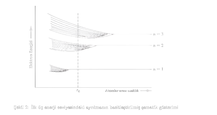
For crystals containing on the order of $10^{20}$ electrons, the energy separation between the split levels is so small that, for practical purposes, the resulting band structure is considered quasi-continuous.

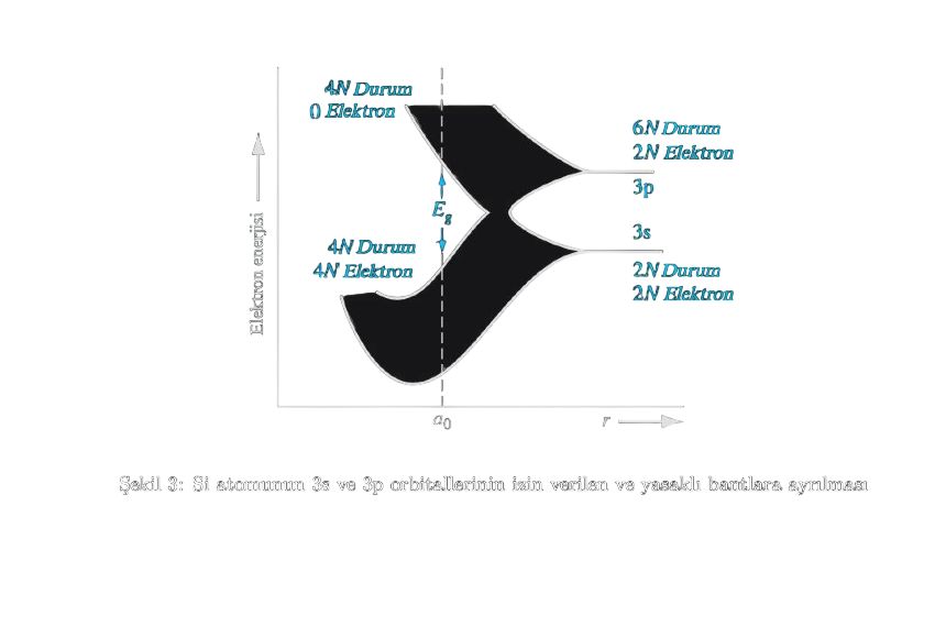
As an example, consider silicon. Ten of its 14 electrons fill the $n=1$ and $n=2$ levels and are strongly bound to the nucleus. The four electrons at $n=3$ are more weakly bound. These outer-shell electrons comprise two in the $3s$ orbital and two in the $3p$ orbital. As Si atoms approach, their $3s$ and $3p$ orbitals overlap first. The resulting overlap reorganizes the eight quantum states—two in $3s$ and six in $3p$—into two bands, four lower-energy and four higher-energy states, as shown in Figure 3. At absolute zero, all states in the lower-energy band are occupied while the higher-energy band is empty. The lower band is called the valence band and the higher band the conduction band. Their characteristic properties are discussed later in this article.

The Kronig–Penney Model

The preceding section treated qualitatively the distribution of allowed electron energies as atoms form a crystal. Quantum mechanics and the Schrödinger wave equation allow the concepts of allowed and forbidden energy bands to be developed in greater detail. The Kronig–Penney model adapts quantum mechanics’ single-potential-well problem to solid-state physics—that is, to a periodic crystal.

The model has two principal aims:

1. To determine how an electron behaves in a periodic potential
2. To see how allowed energy bands and forbidden band gaps arise

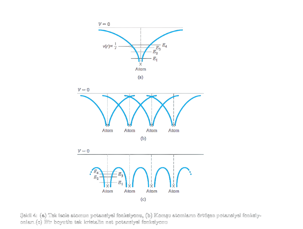
In a real crystal, the potential-energy field is very strong near positively charged ionic cores, forming wells that tend toward negative infinity, and weaker between atoms. Solving this realistic situation in the Schrödinger equation is nearly impossible. To make it tractable, Kronig and Penney replaced the real periodic potential with a periodic series of square-wave potentials. The model is therefore a highly simplified, idealized one-dimensional version of a real crystal.

Figure 4(a) shows the potential of a single, noninteracting one-electron atom and its allowed discrete energy levels. Panel (b) shows the same type of potential for several neighboring atoms in a one-dimensional chain. Finally, neighboring atomic potentials overlap, producing the net potential in (c). This is the potential used in the Schrödinger equation to model a one-dimensional single crystal.

Kronig and Penney model the electron’s motion through a crystal of regularly spaced ionic cores as follows:

• The potential repeats periodically; each cell contains a well and a barrier. Let $a$ be the free-motion region, $b$ the barrier width, and $(a+b)$ the period:
• Well Regions $(0 < x < a)$: The potential energy is zero $(V = 0)$. The electron is relatively free here; this may be viewed as the interior or vicinity of the atomic core.
• Barrier Regions $(-b < x < 0)$: The potential energy is constant $(V = V_0)$. This is the barrier the electron must cross to move from one atom to another.
• Period $(a+b)$: This represents the crystal lattice constant. The potential repeats every $a+b$: $V(x) = V(x+a+b)$.

The time-independent Schrödinger equation for the electron in one dimension is

$$-\frac{\hbar^2}{2m}\frac{d^2\psi(x)}{dx^2} + V(x)\psi(x) = E\psi(x) \tag{1}$$

Because the potential is piecewise, we solve each region separately.

I—Free Region

$$V(x) = 0$$ $$\frac{d^2\psi(x)}{dx^2} + \alpha^2\psi(x) = 0$$

where $\alpha^2 = \dfrac{2mE}{\hbar^2}$. The solution is

$$\psi_{I}(x) = Ae^{i\alpha x} + Be^{-i\alpha x}$$

This is the plane-wave solution.

II—Barrier Region

$$V(x) = V_0$$

If $E < V_0$,

$$\frac{d^2\psi(x)}{dx^2} - \beta^2\psi(x) = 0$$

where $\beta^2 = \dfrac{2m(V_0 - E)}{\hbar^2}$. The solution is

$$\psi_{II}(x) = Ce^{\beta x} + De^{-\beta x}$$

This is the exponentially decaying solution, describing tunneling.

---

We now invoke Bloch’s theorem, which says that the wave function of an electron moving in a periodic potential is the product of a plane wave and a function $u(x)$ carrying the crystal’s periodicity:

$$\psi(x) = u(x)e^{ikx} \tag{2}$$

Because the function is periodic,

$$u_k(x+d) = u_k(x)$$

Here, $k$ is the propagation constant and $u(x)$ has period $a+b$.

As we recall, the complete wave-equation solution is the product of its time-independent and time-dependent solutions:

$$\Psi(x,t) = \psi(x)\phi(t) = u(x)e^{ikx} \cdot e^{-i\left(\frac{E}{\hbar}\right)t} \tag{3}$$

It can also be written as

$$\Psi(x,t) = u(x)e^{i\left(kx - \left(\frac{E}{\hbar}\right)t\right)} \tag{4}$$

This traveling-wave solution describes an electron moving through a single crystal. The wave amplitude is periodic, and $k$ is called the wave number. We can now relate $k$, $E$, and $V_0$.

In region I of Figure 5, where $(0 < x < a)$ and $V(x) = 0$, taking the second derivative of equation (2) and substituting it into the time-dependent Schrödinger equation gives

$$\frac{d^2u_1(x)}{dx^2} + 2ik\frac{du_1(x)}{dx} - (k^2 - \alpha^2)u_1(x) = 0 \tag{5}$$

Here $u_1(x)$ is the wave-function amplitude in region I, and $\alpha$ is, as defined above,

$$\alpha^2 = \frac{2mE}{\hbar^2} \tag{6}$$

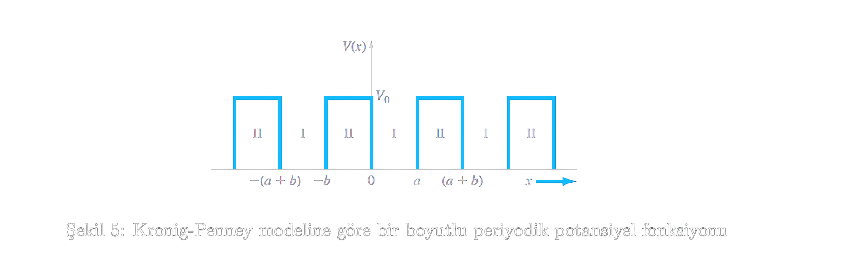
In region II, $-b < x < 0$ and $V(x) = V_0$. Applying the Schrödinger equation gives

$$\frac{d^2u_2(x)}{dx^2} + 2ik\frac{du_2(x)}{dx} - \left(k^2 - \alpha^2 + \frac{2mV_0}{\hbar^2}\right)u_2(x) = 0 \tag{7}$$

Here $u_2(x)$ is the wave-function amplitude in region II. We define the parameter relation as

$$\frac{2m}{\hbar^2}(E - V_0) = \alpha^2 - \frac{2mV_0}{\hbar^2} = \beta^2 \tag{8}$$

Equation (7) can therefore be rewritten as

$$\frac{d^2u_2(x)}{dx^2} + 2ik\frac{du_2(x)}{dx} + (k^2 - \beta^2)u_2(x) = 0 \tag{9}$$

Notice that in equation 8, $\beta$ is real if $E > V_0$ and imaginary if $E < V_0$.

The region-I solution of equation 5 is

$$u_1(x) = Ae^{i(\alpha - k)x} + Be^{-i(\alpha + k)x}, \quad 0 \le x \le a \tag{10}$$

of this form.

The region-II solution of equation 9 is

$$u_2(x) = Ce^{i(\beta - k)x} + De^{-i(\beta + k)x}, \quad -b \le x \le 0 \tag{11}$$

of this form. Since $V(x)$ is finite everywhere, the wave function $\psi(x)$ and its first derivative $\frac{\partial\psi(x)}{\partial x}$ must be continuous. This also requires the amplitude $u(x)$ and its first derivative $\frac{\partial u(x)}{\partial x}$ to be continuous.

Considering the boundary at $x = 0$ and applying continuity to the amplitude,

$$u_1(0) = u_2(0) \tag{12}$$

substitution of equations 10 and 11 into equation 12 gives

$$A + B - C - D = 0 \tag{13}$$

Now apply the next condition:

$$\left.\frac{du_1}{dx}\right|_{x=0} = \left.\frac{du_2}{dx}\right|_{x=0} \tag{14}$$

This yields

$$(\alpha - k)A - (\alpha + k)B - (\beta - k)C + (\beta + k)D = 0 \tag{15}$$

We defined region I as $(0 < x < a)$ and region II as $(-b < x < 0)$. Periodicity and continuity mean that $u_1$ as $x \rightarrow a$ equals $u_2$ as $x \rightarrow -b$. Thus $u_1(a) = u_2(-b)$. Applying the solutions for $u_1(x)$ and $u_2(x)$ to this boundary condition gives

$$Ae^{i(\alpha - k)a} + Be^{-i(\alpha + k)a} - Ce^{-i(\beta - k)b} - De^{i(\beta + k)b} = 0 \tag{16}$$

Our final boundary condition is

$$\left.\frac{du_1}{dx}\right|_{x=a} = \left.\frac{du_2}{dx}\right|_{x=-b} \tag{17}$$

which yields

$$(\alpha - k)Ae^{i(\alpha - k)a} - (\alpha + k)Be^{-i(\alpha + k)a} - (\beta - k)Ce^{-i(\beta - k)b} + (\beta + k)De^{i(\beta + k)b} = 0 \tag{18}$$

The four boundary conditions have now produced four homogeneous equations—13, 15, 16, and 18—in four unknowns. A simultaneous linear homogeneous system has a nonzero solution if and only if the determinant of its coefficients is zero. Here, the coefficients multiply $A, B, C$, and $D$. We will not work through this lengthy $4 \times 4$ determinant; detailed treatments are listed in the references. The result is

$$\cos k(a+b) = \frac{-(\alpha^2 + \beta^2)}{2\alpha\beta}(\sin\alpha a)(\sin\beta b) + (\cos\alpha a)(\cos\beta b) \tag{19}$$

Equation (19) relates $k$ to the total energy $E$ through $\alpha$, and to $V_0$ through $\beta$.

As noted, the more interesting solutions arise for $E < V_0$, corresponding to an electron bound within the crystal. Then $\beta$ is imaginary. Defining a real quantity $\gamma$ by

$$\beta = i\gamma \tag{20}$$

equation (19) becomes

$$\frac{\gamma^2 - \alpha^2}{2\alpha\gamma}(\sin\alpha a)(\sinh\gamma b) + (\cos\alpha a)(\cosh\gamma b) = \cos k(a+b) \tag{21}$$

Equation (21) has no analytic solution, so it must be solved numerically or graphically to obtain the relation among $k$, $E$, and $V_0$. Solving the Schrödinger equation for a single bound particle produced discrete allowed energies; solving equation (21) instead produces a band of allowed energies. To obtain an equation more amenable to graphical solution and thus better reveal the nature of the results, take the limits $b \rightarrow 0$ and $V_0 \rightarrow \infty$ while keeping the product $bV_0$ finite. Equation (3.21) then reduces to

$$\left(\frac{mV_0 ba}{\hbar^2}\right)\frac{\sin\alpha a}{\alpha a} + \cos\alpha a = \cos ka \tag{22}$$

We can define $P'$ as

$$P' = \frac{mV_0 ba}{\hbar^2} \tag{23}$$

Finally, we obtain

$$P'\frac{\sin\alpha a}{\alpha a} + \cos\alpha a = \cos ka \tag{24}$$

Equation (24) again relates $k$, the total energy $E$ through $\gamma$, and the potential barrier $bV_0$. Note that equation (24) is not itself a direct solution of the Schrödinger equation; rather, it states the conditions necessary for a solution. If the crystal is assumed infinite, $k$ in equation (24) can vary continuously and must be real.

The k-Space (Wave-Vector Space) Diagram

To understand the nature of our solution, first consider $V_0 = 0$. Then $P' = 0$; with no potential barrier, this corresponds to a free particle. Equation (24) gives

$$\cos\alpha a = \cos ka \tag{25}$$

or

$$\alpha = k \tag{26}$$

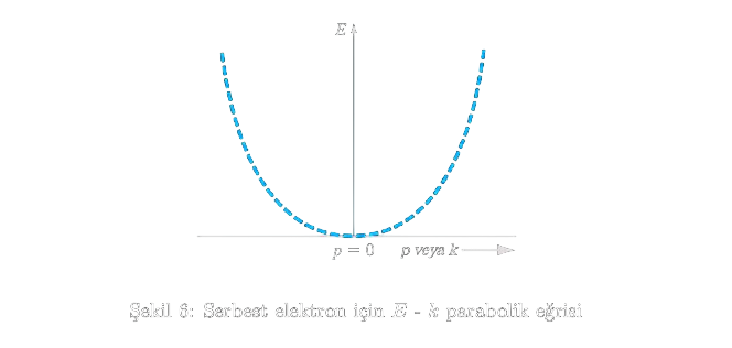
Because the potential is zero, total energy $E$ equals kinetic energy. Therefore,

$$\alpha = \sqrt{\frac{2mE}{\hbar^2}} = \sqrt{\frac{2m\left(\frac{1}{2}mv^2\right)}{\hbar^2}} = \frac{p}{\hbar} = k \tag{27}$$

Here $p$ is the particle momentum. For a free electron, the propagation constant $k$ is related to momentum. This parameter is also called the wave number and, by the de Broglie relation, is defined as

$$k = \frac{p}{\hbar} \tag{3.27}$$

The energy–momentum relation is

$$E = \frac{p^2}{2m} = \frac{\hbar^2 k^2}{2m} \tag{28}$$

Figure 6 shows the parabolic relation between energy $(E)$ and momentum $(p)$ in equation (28) for a free particle. Since momentum and wave number are linearly related, Figure 6 is also the free-particle $E-k$ diagram. Now consider the relation between $E$ and $k$ obtained from equation (24) for a particle in a single-crystal lattice. As $P'$ increases, the particle becomes more tightly bound to the potential well or atom. We can define the left-hand side of equation (24) as a function $f(\alpha a)$:

$$f(\alpha a) = P'\frac{\sin\alpha a}{\alpha a} + \cos\alpha a \tag{29}$$

Figure 7a plots the first term of equation (29) against $\alpha a$; Figure 7b plots $\cos\alpha a$; and Figure 7c plots their sum, $f(\alpha a)$. Equation (24) also gives

$$f(\alpha a) = \cos\alpha a \tag{30}$$

For equation (30) to hold, $f(\alpha a)$ must lie between $-1$ and $+1$, since cosine cannot lie outside that interval. In Figure 7c, the allowed values of $f(\alpha a)$ and the corresponding intervals of $\alpha a$ are shaded. The figure also shows the values of $ka$ from the right-hand side of equation (30) that correspond to the allowed values of $f(\alpha a)$.

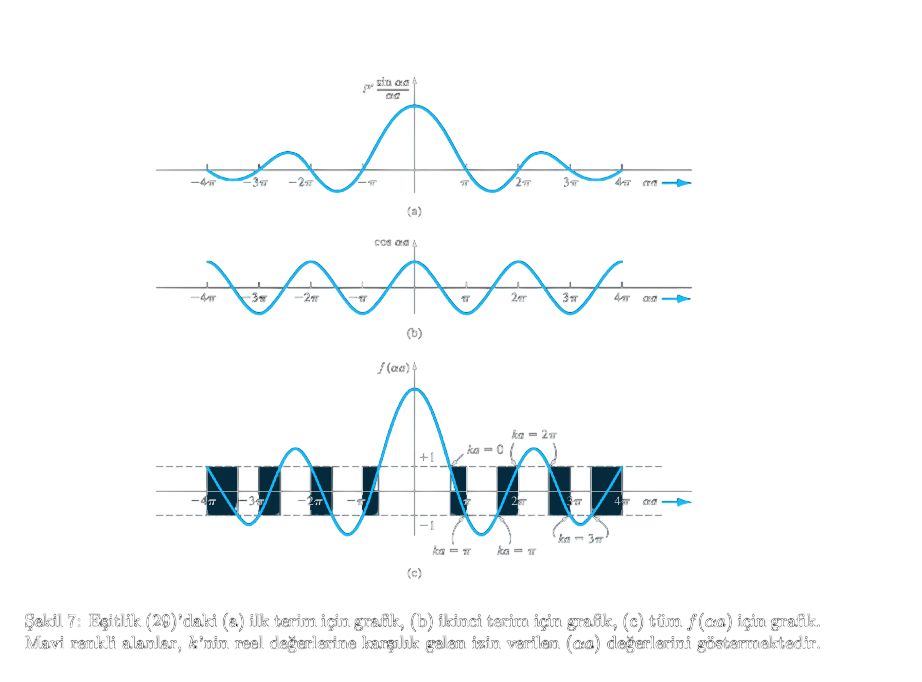
The parameter $\gamma$ is related to the particle’s total energy $E$ by

$$\gamma^2 = \frac{2mE}{\hbar^2}$$

Using Figure 7c, we can plot the particle energy $E$ as a function of wave number $k$. Figure 8 shows this graph and thereby reveals the allowed energy bands for a particle traveling through a crystal lattice. Discontinuities in $E$ also produce forbidden energy ranges for particles in the crystal.

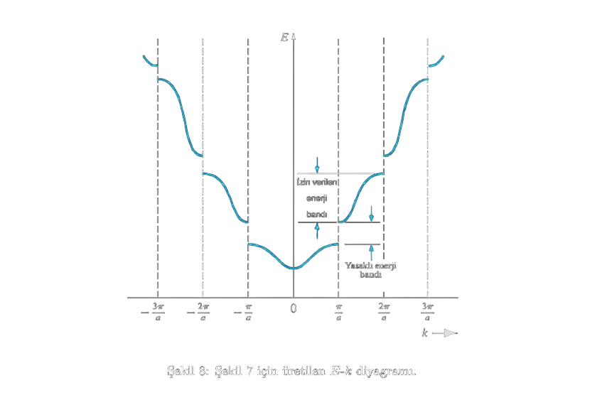
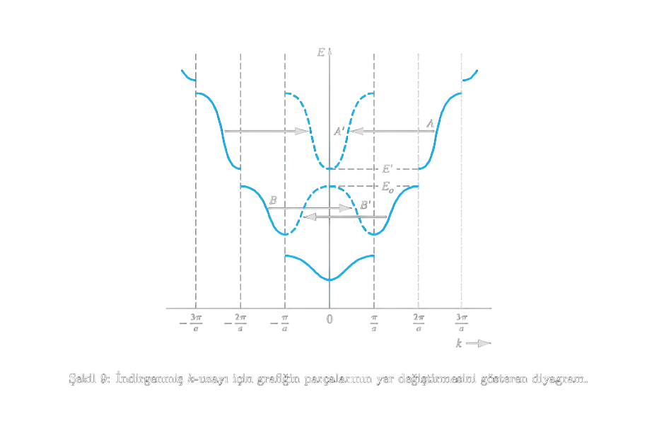
Consider again the right-hand side of equation (24), $\cos ka$. Since cosine is periodic, for positive integer $n$ we may write

$$\cos ka = \cos(ka + 2n\pi) = \cos(ka - 2n\pi) \tag{31}$$

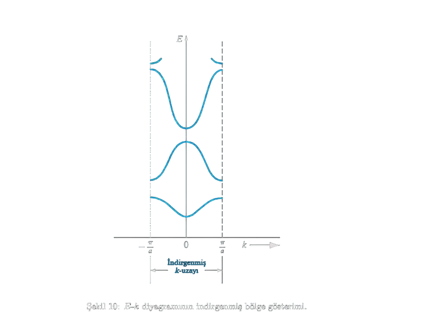
With Figure 8 in mind, particular portions of the curve may be shifted by $2\pi$ while equation (24) remains satisfied. Figure 9 shows how various segments can be shifted by a factor of $2\pi$. Figure 10 shows the entire $E-k$ diagram collected within $-\frac{\pi}{a} \le k \le \frac{\pi}{a}$. This is called the reduced k-space diagram or reduced-zone representation.

In equation (27), we stated that for a free electron, momentum and wave number obey $p = \hbar k$. Given the similarity between the free-electron solution and the single-crystal results in Figure 8, $k$ in a single crystal is called crystal momentum. It is not the electron’s actual momentum within the crystal, but a propagation constant that also incorporates the crystal interaction.

Thus far, we have examined the Kronig–Penney model, a one-dimensional periodic potential used to model a single-crystal lattice. The central result is that electrons in a crystal occupy particular allowed energy bands and are excluded from forbidden bands. A similar energy-band theory applies to real three-dimensional single crystals. In subsequent parts, we will use the Kronig–Penney model to derive further properties of the electron.