Semiconductor Physics Series, Part 2: A Little Quantum Mechanics

Introduction

In the second part of our semiconductor physics series, we will briefly examine the quantum-mechanical processes needed to understand the band structures that give semiconductor materials their functionality, and see how properties of an electron in a potential, such as its energy and position, differ from those of classical objects. By theoretically treating the electron as a discrete, isolated system, this part lays the groundwork for the larger systems we will encounter later. It should be kept in mind, however, that the concepts discussed here require far more detailed analysis and can only be presented in summary form in a series whose primary purpose is not to explain the foundations of quantum mechanics. We can begin with a brief history.

Historical Background

The cathode-ray experiments conducted by J. J. Thomson following the discovery of the electron in 1897 led to the acceptance of the idea that electrons were classical particles. Later experiments, however, such as those on blackbody radiation, began to overturn the prevailing belief that energy was continuous. Physicists began adopting a new approach that could resolve experimental contradictions by using discrete entities first proposed by Max Planck and called energy quanta. Although this approach could account for light in the photoelectric effect, understanding electrons took longer. By around 1913, radiation at specific frequencies observed in electron-excitation experiments—in other words, a discrete spectrum—gave rise to the idea of specific orbits with distinct energy levels, as in the Bohr model, strengthening the view that the electron was not a classical particle. The de Broglie hypothesis, proposed by L. de Broglie in 1924, extended wave–particle duality to material bodies and demonstrated the mathematical consistency of the idea; roughly three years later, the electron-diffraction experiment conducted by Davisson and Germer proved that electrons also exhibit this duality. The limitations of the astronomically inspired orbital picture then prompted scientists to seek a new method. The theoretical frameworks that met this need and are regarded as the beginning of modern quantum mechanics were W. Heisenberg’s energy and momentum relations, developed in 1925, and the wave mechanics introduced by E. Schrödinger in 1926.

Energy Quanta

The idea that energy is emitted in discrete packets was first proposed in 1900 by the German physicist Max Planck. Building on L. Boltzmann’s statistical approach, Planck described the thermal radiation emitted by a heated surface in terms of discrete packets of energy called “quanta.” According to this description, the energy carried by these packets is

$$E=h\nu \tag{1}$$

where $E$ is energy, $\nu$ is the frequency of the radiation, and $h$ is Planck’s constant.

Only a few years later, in 1905, Einstein developed a model that explained the photoelectric effect through a similar energy-quantum approach. This model states that the energy in a light wave is also emitted in discrete packets called “photons.”

Wave–Particle Duality

The de Broglie hypothesis is a fundamental concept of quantum mechanics developed by Louis de Broglie in 1924. It extends the wave–particle duality of light to particles of matter such as electrons and protons.

According to the de Broglie hypothesis, every object also has a de Broglie wavelength. Although this wavelength is too small to detect on macroscopic scales, it produces observable quantum effects on subatomic scales. The de Broglie wavelength is inversely proportional to the particle’s momentum, and this relation is written as

$$\lambda=h/p \tag{2}$$

where $\lambda$ is the wavelength, $h$ is Planck’s constant, and $p$ is momentum.

In 1927, the electron-diffraction experiment performed by Davisson and Germer using single-crystal nickel¹ provided experimental evidence for the electron’s dual nature through the interference pattern produced by nickel’s periodic atomic arrangement.

Uncertainty Principle

The Heisenberg uncertainty principle states that conjugate quantities such as momentum and position, or energy and time, cannot be measured simultaneously with absolute precision. Measuring one entails uncertainty in the other.

If $\Delta p$ is the uncertainty in momentum and $\Delta x$ is the uncertainty in position, then

$$\Delta p \Delta x \ge \hbar \tag{3}$$

Here, $\hbar: h/2{\pi}$ is the reduced Planck constant.

$$\hbar=1.054\cdot 10^{-34}js \tag{4}$$

Similarly, with $\Delta E$ denoting the uncertainty in energy and $\Delta t$ the uncertainty in time,

$$\Delta E \Delta t \ge \hbar \tag{5}$$

The Heisenberg uncertainty principle does not point to inadequacies in measurement techniques; rather, it expresses a fundamental fact about the probabilistic nature of the quantum world. One of its most important consequences is that the electron is represented as a probability cloud around an atomic nucleus. In other words, we calculate the probability of finding the electron at a particular position. Semiconductor technologies essentially work by manipulating this probability distribution to obtain the desired electrical properties.

Schrödinger’s Wave Equation

The wave equation, a fundamental postulate of quantum mechanics, is written as follows.

$${\frac{-\hbar^2}{2m}}\cdot{\frac{\partial^2 \Psi(x,t)}{\partial x^2}} + V(x)\Psi(x,t)= j\hbar \frac{\partial \Psi(x,t)}{\partial t} \tag{6}$$

The wave function $\Psi(x,t)$ in this equation provides important information about a physical system composed of particles. In addition, $V(x)$ denotes the time-independent potential, $m$ the mass of the particle, and $j$ the imaginary unit.

The first method we can apply to extract meaningful results from this differential equation is separation of variables. Here, the wave function is written as the product of two functions, one depending only on time and the other only on position.

$$\Psi(x,t)= \psi(x) \phi(t) \tag{7}$$

Substituting the wave function in (7) into the wave equation in (6) and dividing both sides by the wave function gives

$${\frac{-\hbar^2}{2m} \frac{1}{\psi(x)} {\frac{\partial^2 \psi(x)}{\partial x^2}}} + V(x)= j\hbar \cdot \frac{1}{\phi(t)} \cdot {\frac{\partial \phi(t)}{\partial t}} \tag{8}$$

Because the left-hand side is a function only of position and the right-hand side only of time, both must equal a constant. Taking $\eta$ as the separation constant, the time-dependent part is

$$\eta = j\hbar \cdot \frac{1}{\phi(t)} \cdot {\frac{\partial \phi(t)}{\partial t}} \tag{9}$$

The solution of differential equation (9) is

$$\phi(t) = e^{-j (\eta/\hbar) t} \tag{10}$$

Since $E=h\nu={h\omega}/{2\pi}$, the angular frequency is $\omega = {\eta}/{\hbar}=E/\hbar$
Thus, our separation constant equals the energy.

Using this information, the position-dependent part of equation (8) can be written as

$$\frac{\partial^2 \psi(x)}{\partial x^2} + \frac{2m}{\hbar^2}(E-V(x))\psi(x) = 0 \tag{11}$$

Finally, the general wave function is

$$\Psi(x,t)= \psi(x)\phi(t)= \psi(x) e^{-j(E/\hbar)t} \tag{12}$$

The squared absolute value of this deceptively simple function determines the probability distribution of a particle’s position.

We will now use the time-independent wave equation to examine the electron under different potentials.

Electron in Free Space

Let us begin with the simplest possible hypothetical situation: one in which no net force acts on the electron. In other words, the electron moves under a constant potential $V(x)$. For convenience, assume $V(x)=0$ for all $x$. The time-independent wave equation then becomes

$$\frac{\partial^2 \psi(x)}{\partial x^2} + \frac{2mE}{\hbar^2}\psi(x)=0 \tag{13}$$

Taking $k$ as the wave number and A and B as coefficients, the solution is

$$\psi(x)=A exp(jkx)+B exp(-jkx) \tag{14}$$ $$k=\sqrt{\frac{2mE}{\hbar}} \tag{15}$$

Now let us use the time-dependent solution in equation (10) to rewrite the general wave equation:

$$\Psi(x,t)=A exp[j(kx-wt)]+B exp[-j(kx+wt)] \tag{16}$$

The result in (16) has the mathematical form of a traveling wave. The first term, with coefficient $A$, represents a wave traveling in the +$x$ direction, while the second, with coefficient $B$, represents a wave traveling in the -$x$ direction.

Let us continue by conventionally considering the wave traveling in the +$x$ direction. The wave number $k$ is

$$k=\sqrt{\frac{2mE}{\hbar^2}}=\sqrt{\frac{p^2}{\hbar^2}}=\frac{p}{\hbar} \tag{17}$$

Using the de Broglie wavelength relation, we obtain

$$k=\frac{2\pi}{\lambda} \tag{18}$$

Thus, the free electron has a well-defined momentum.

Moreover, the probability density function $\Psi(x,t)\Psi^*(x,t)= AA^*$ is a constant independent of position. Physically, a free electron with well-defined momentum is equally likely to be found at any point in space. This agrees with the Heisenberg uncertainty principle, because well-defined momentum implies uncertainty in position.

Infinite Potential Well

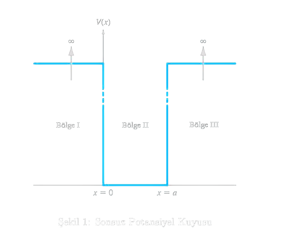
The infinite potential well is the most elementary model in which an electron is confined by a specified potential. As shown in Figure 1, the electron is confined to region II between two infinitely high potential barriers.

Recalling the time-independent part of the wave equation (11):

$$\frac{\partial^2 \psi(x)}{\partial x^2} + \frac{2m}{\hbar^2}(E-V(x))\psi(x) = 0 \tag{19}$$

Because the energy $E$ is finite, the wave function $\psi(x)$ must vanish in regions I and III, where the potential is infinite. Thus, the probability of finding the electron in either region is zero.

In region II, the potential $V$ is zero, so the time-independent wave equation becomes

$$\frac{\partial^2 \psi(x)}{\partial x^2} + \frac{2mE}{\hbar^2}\psi(x) = 0 \tag{20}$$

A particular solution is

$$\psi(x)=A_1cos(kx)+A_2sin(kx) \tag{21}$$ $$k=\sqrt{\frac{2mE}{\hbar^2}} \tag{22}$$

Applying the boundary condition that $\psi(x)$ be continuous,

$$\psi(x=0)=\psi(x=a)=0 \tag{23}$$

we find $A_1=0$, and at $x=a$

$$A_2sin(ka)=0 \tag{24}$$

Thus, for positive integer $n$, the wave number $k$ is

$$k=\frac{n\pi}{a} \tag{25}$$

Now let us determine $A_2$ using the other boundary condition, normalization. Since $\psi(x)$ is real here, we use $\psi(x)=\psi^*(x)$.

$$\int_0^a A_2^2sin^2(kx) \,dx = 1 \tag{26}$$ $$A_2=\sqrt{\frac{2}{a}} \tag{27}$$

Consequently, for positive integer n, the time-independent wave function takes the form

$$\psi(x)=\sqrt{\frac{2}{a}}sin\left(\frac{n\pi x}{a}\right) \tag{28}$$

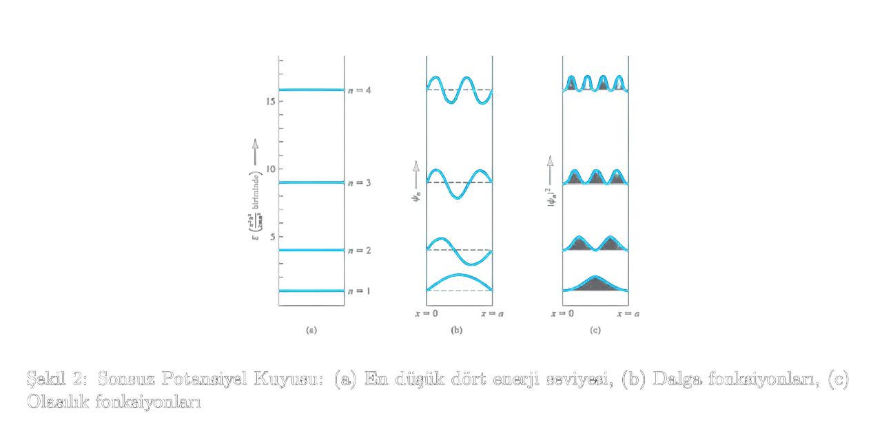
The free electron in the preceding section was represented by a traveling wave. This equation instead shows that a bound electron is represented by a standing wave. Finally, using equations (25) and (28), let us examine the relation between wave number $k$ and total energy $E$.

$$k_n^2=\frac{2mE_n}{\hbar^2}=\frac{n^2\pi^2}{a^2} \tag{29}$$ $$E=E_n=\frac{\hbar^2 n^2 \pi^2}{2ma^2} \tag{30}$$

This example mathematically demonstrates that an electron behaves in a localized manner under certain potentials. We must also conclude that a bound electron has discrete energy levels. For the infinite potential well, these levels are shown in Figure 2. We will discuss these energy levels and the probability-distribution function in detail later.

Let us now make the example more realistic by considering a finite potential.

Potential Barrier and Tunneling

The penetration of potential barriers by quantum wave functions was first studied theoretically by F. Hund in 1927. Soon afterward, Schrödinger’s wave equation enabled certain radioactive decays previously regarded as classically impossible, such as $\alpha$ decay, to be explained through tunneling. The tunnel diode, invented by Leo Esaki in 1957, showed that tunneling is observable not only in atomic nuclei but also in semiconductors. Applications of quantum tunneling diversified greatly between 1960 and 1990, playing an important role throughout nanotechnology, from measurement technologies and superconductors to quantum computers.

The simplest system for describing quantum tunneling is the finite-height square potential barrier in Figure 3. It is expressed as

$$U(x)= \begin{cases} 0,\ x<0 \\ U_0,\ 0\le x \le L \\ 0,\ x>L \end{cases} \tag{31}$$

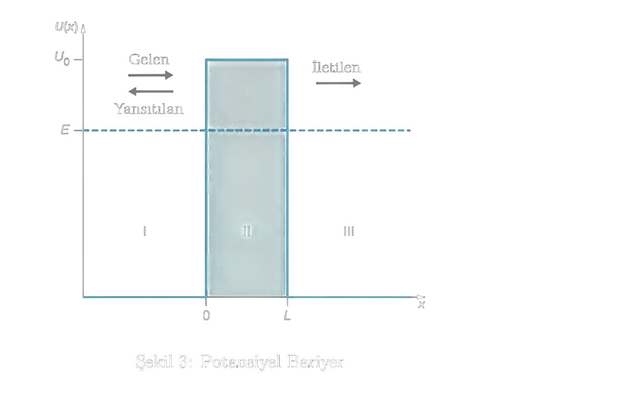
Suppose that a time-independent electron beam with energy $E$ is directed toward the barrier along the +$x$ direction. Recalling the time-independent wave equation,

$$\frac{-\hbar^2}{2m} \frac{d^2\psi(x)}{dx^2}+U(x)\psi(x)=E\psi(x) \tag{32}$$

Let $\psi_I(x)$, $\psi_{II}(x)$, and $\psi_{III}(x)$ denote the wave functions in regions I, II, and III, respectively, in Figure 3. The time-independent wave equation can then be written for each region as follows:

$$\frac{-\hbar^2}{2m} \frac{d^2\psi_I(x)}{dx^2}=E\psi_I(x)\quad ,-\infty<x<0 \tag{33}$$

$$\frac{-\hbar^2}{2m}\frac{d^2\psi_{II}(x)}{dx^2}+U_0\psi_{II}(x)=E\psi_{II}(x)\quad , 0\le x\le L \tag{34}$$ $$\frac{-\hbar^2}{2m}\frac{d^2\psi_{III}(x)}{dx^2}=E\psi_{III}(x)\quad , L<x<+\infty \tag{35}$$

Our function must be continuous, so the boundary conditions are

$$\psi_I(0)=\psi_{II}(0) \tag{36}$$ $$\psi_{II}(L)=\psi_{III}(L) \tag{37}$$

The first derivatives of the wave functions must also be continuous at the region boundaries:

$$\left. \frac{d\psi_I(x)}{dx} \right |_{x=0}= \left. \frac{d\psi_{II}(x)}{dx} \right |_{x=0} \tag{38}$$ $$\left. \frac{d\psi_{II}(x)}{dx} \right |_{x=L}= \left. \frac{d\psi_{III}(x)}{dx} \right |_{x=L} \tag{39}$$

The wave functions in regions I and II are as follows.

$$\psi_I(x)=Ae^{+ikx}+Be^{-ikx} \tag{40}$$ $$\psi_{III}(x)=Fe^{+ikx}+Ge^{-ikx} \tag{41}$$

Here, $k=\sqrt{2mE}/\hbar$.

Region I contains an incident and a reflected wave, represented by the terms with coefficients $A$ and $B$ in equation 40. Region III, however, contains only the transmitted wave; hence $G=0$.

Using these equations, the tunneling probability for a particle incident on the barrier can be written as

$$T(L,E)=\frac{|\psi_{tra}(x)|^2}{|\psi_{in}(x)|^2}=\frac{|F||F|^*}{|A||A|^*}=\left |\frac{F}{A}\right |^2 \tag{42}$$

Here, $L$ is the barrier width and $E$ is the particle’s total energy.

For region II, equation 34

$$\frac{d^2\psi_{II}(x)}{dx^2}=\beta^2\psi_{II}(x) \tag{43}$$ $$\beta^2=\frac{2m}{\hbar^2}(U_0-E) \tag{44}$$

can be rewritten as

$$\psi_{II}(x)=Ce^{-\beta x}+ De^{+\beta x} \tag{45}$$

is its solution.

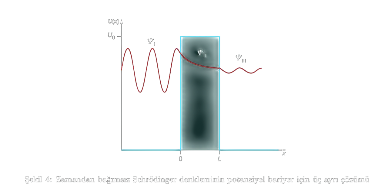
As can be seen, the wave function in region II is not oscillatory but decays progressively.

The solutions in all three regions are illustrated in Figure 4.

Using the information in equations 45, 46, 47, and 48, the ratio $F/A$,

$$\gamma = \beta/k\ - k/\beta \tag{46}$$

with

$$\frac{F}{A}=\frac{e^{-ikL}}{cosh(\beta L)+i(\gamma /2)sinh(\beta L)} \tag{47}$$

is found to be

Thus, using equation 42, we obtain

$$T(L,E)=16\frac{E}{U_0}\left(1-\frac{E}{U_0}\right)e^{-2\beta L} \tag{48}$$

This example showed how tunneling allows an electron to cross a potential whose energy exceeds the electron’s own. Although impossible in classical physics, this behavior yields testable and consistent results on the quantum scale.

Extending Wave Theory to Simple Atoms

Thus far, we have considered only simplified two-dimensional systems. Before concluding, let us revisit the wave equation in three dimensions for a one-electron atom such as hydrogen and briefly discuss quantum numbers.

For hydrogen, the potential is the Coulomb potential,

$$V(r)=\frac{-e^2}{4\pi \epsilon_0 r} \tag{49}$$

Here, $e$ is the magnitude of the electron’s charge, $\epsilon_0$ the permittivity of free space, and $r$ the electron’s radial distance from the nucleus. Since the potential is spherically symmetric, we rewrite the time-independent wave function in spherical coordinates.

$$\nabla^2 \psi(r,\theta,\phi)+\frac{2m_0}{\hbar^2}(E-V(r))\psi(r,\theta,\phi)=0 \tag{50}$$

Writing the Laplacian in spherical coordinates allows the wave equation

$$\frac{1}{r^2}\cdot \frac{\partial}{\partial r} \left(r^2 \frac{\partial \psi}{\partial r}\right)+\frac{1}{r^2 sin^2 \theta}\cdot \frac{\partial^2\psi}{\partial \phi^2}+\frac{1}{r^2 sin\theta}\cdot \frac{\partial}{\partial \theta}\left(sin\theta \cdot \frac{\partial \psi}{\partial \theta}\right)+\frac{2m_0}{\hbar^2}(E-V(r))\psi=0 \tag{51}$$

to be rewritten as follows.

Let us apply separation of variables.

$$\psi(r,\theta,\phi)=R(r)\cdot \Theta(\theta)\cdot \Phi(\phi) \tag{52}$$

Our new wave equation is

$$\frac{sin^2\theta}{R}\cdot \frac{\partial}{\partial r}\left(r^2\frac{\partial R}{\partial r}\right)+\frac{1}{\Phi}\cdot \frac{\partial^2 \phi}{\partial \phi^2}+\frac{sin\theta}{\Theta}\cdot \frac{\partial}{\partial\theta}\left(sin\theta \cdot\frac{\partial \Theta}{\partial \theta} \right)+r^2sin^2\theta\cdot \frac{2m_0}{\hbar^2}(E-V)=0 \tag{53}$$

Because the second term in equation 53 depends only on $\phi$, let us examine it first. Taking $m$ as the separation constant,

$$\frac{1}{\Phi}\cdot \frac{\partial^2\Phi}{\partial \phi^2}=-m^2 \tag{54}$$

the solution for $\phi$ is

$$\Phi(\phi)=e^{jm\phi} \tag{55}$$

In this case,

$$\Phi(\phi+2\pi)=\Phi(\phi) \tag{56}$$

Thus, $m$ must be an integer.

$$m=0,\ \pm 1, \ \pm2, \ ... \tag{57}$$

Similarly, separation constants and complex algebraic manipulations yield the angular and radial solutions, $\Theta(\theta)$ and $R(r)$, respectively. Writing them requires functions such as Legendre polynomials and spherical Bessel functions, together with an extended potential called the effective potential. We will not pursue these calculations here.²

The electron’s energy is

$$E_n=\frac{-m_0e^4}{(4\pi \epsilon_0)^22\hbar^2n^2} \tag{58}$$

defined in this way.

The quantum numbers obtained through the algebraic analysis are listed in Table 1.

Symbol	Name	Range of Values
$n$	Principal quantum number	$1, 2, 3, ...$
$l$	Orbital angular-momentum quantum number	$0,1,2,...,n-1$
$m$	Magnetic quantum number	$-l,...,0,...,+l$

Table 1. Quantum Numbers

All quantities in Table 1 are derived from the system’s boundary conditions and symmetry. Each quantum number is an eigenvalue corresponding to a quantum operator and represents an observable. The principal quantum number $n$ emerges from the radial solution of Schrödinger’s wave equation and provides information about the electron’s energy levels and orbital radii. The orbital angular-momentum quantum number $l$ is obtained by separating the angular components of the wave equation in spherical coordinates and provides information about the orbital’s angular momentum and shape. As shown above, the magnetic quantum number $m$—also written $m_l$ in some sources—is derived from the angular equation and describes the $z$ component of angular momentum, providing information about the orbital’s orientation in space.

The solution of the wave equation is written as $\psi_{nlm}$ in terms of these three quantum numbers.

$$\psi_{nlm}=\sqrt{\left(\frac{2}{na_0}\right)^3\frac{(n-l-1)!}{2n(n+l)!}}e^{-r/na_0} \left(\frac{2r}{na_0}\right)^l [L_{n-l-1}^{2l+1}(2r/na_0)]Y_l^m(\theta,\phi) \tag{59}$$

Here, $n$, $l$, and $m$ are the quantum numbers, $a$ is the Bohr radius, $Y_l^m(\theta,\phi)$ denotes the spherical harmonics, and $L_{n-l-1}^{2l+1}$ is a Laguerre polynomial.

$$a_0=\frac{4\pi \epsilon_0 \hbar^2}{m_0e^2}=0.529 \text{\r{A}} \tag{60}$$

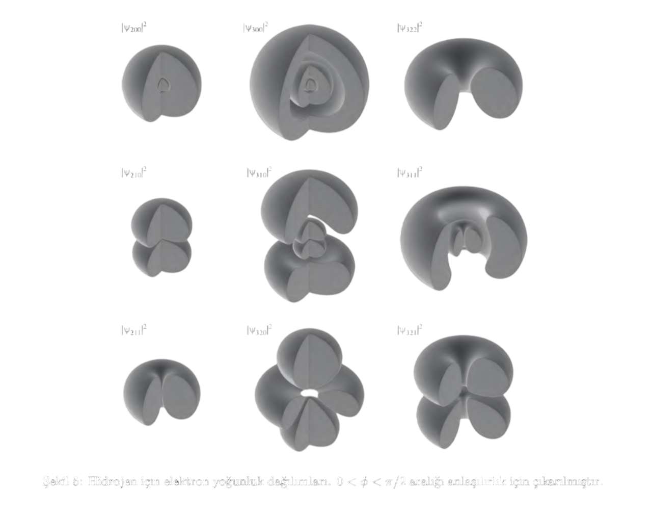
The first few electron-density distributions for hydrogen are plotted in Figure 5.

Another quantum number, not derived from the spatial wave function but associated with the intrinsic spin degree of freedom, is the spin quantum number ($m_s$). It represents the particle’s intrinsic angular momentum and, for an electron, can take only the two values below.

$$m_s=+\frac{1}{2},-\frac{1}{2} \tag{61}$$

Bound electrons in an atom or molecule are described by the four quantum numbers outlined above.

Another concept needed to understand the band structures encountered later is the Pauli exclusion principle. Two identical fermions cannot simultaneously occupy the same quantum state. In other words, two electrons cannot have all four quantum numbers identical. Each orbital can therefore contain at most two electrons with opposite spin orientations. This restriction is the fundamental reason for the band structures discussed in the next part.

In this part, we touched on the electron’s dual nature and the discreteness of its bound-state energy levels while surveying simple potential-well models. We also considered the potential barrier and introduced tunneling. Finally, we used the wave equation to examine hydrogen, discussed quantum numbers, and briefly introduced the Pauli exclusion principle. Although this does not provide a complete understanding of these topics, it lays a foundation for later parts. Next, we will explain the quantum theory of solids and examine the behavior of electrons in solid crystal structures.

References

• Semiconductor Physics And Devices by Donald A. Neamen Third Edition
• Introduction to Quantum Mechanics by D.J. Griffiths and D.F. Schroeter
• Openstax University Physics Volume 3
• https://en.wikipedia.org/wiki/Quantum-number
• https://en.wikipedia.org/wiki/Quantum-mechanics

Footnotes

Footnotes

1. We will discuss the electron-diffraction method, which plays an important role in analyzing crystal structures, in detail in later parts. ↩

2. For a detailed treatment, see: Introduction to Quantum Mechanics, David J. Griffiths and Darrell F. Schroeter ↩