Relativity Series Part 4 - Vectors, Dual Vectors and Tensors

Vectors

To examine the spacetime under consideration in greater detail, we will introduce the concept of a vector. Because we are working in spacetime, our vectors are four-dimensional and, for this reason, are commonly called four-vectors. They have properties different from those of the vectors familiar to us in three dimensions. In the familiar definition, a vector represents the displacement between two points and extends from one point to the other. Such vectors can also be placed head to tail to obtain a new vector. Four-vectors defined on curved spacetime, however, do not possess these properties. Moreover, the vectors we define in spacetime are invariant under all transformations.

Four-vectors live in the tangent space ($T_p$) defined at every point $p$ in spacetime. Consider the curves that can pass through a point $p$ in spacetime. These are smooth curves, meaning that they are continuous and infinitely differentiable from a one-dimensional space into a four-dimensional space. We can parametrize these curves with a parameter such as $\lambda$. Through this parametrization, we define differentiation with respect to that parameter at the point $p$. The derivative of the curve with respect to $\lambda$ at $p$ gives us the vector along that curve. If we define this operation at $p$ for every curve, we define the tangent space at $p$ and all the four-vectors contained in that tangent space.

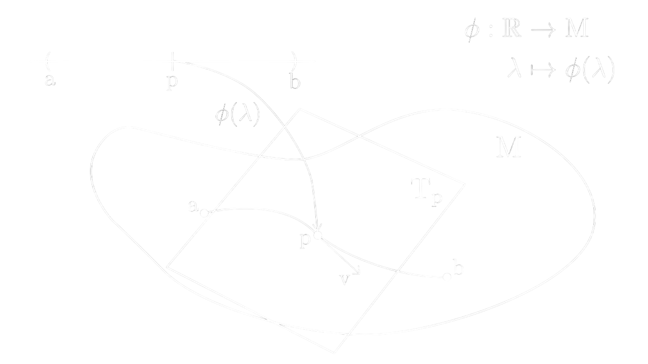
The manifold shown in the figure represents our four-dimensional spacetime. Manifolds are topological spaces that locally possess a Euclidean space at every point and are formed by joining these regions smoothly. A person walking on Earth, for example, would say that the region around them is locally flat; when we examine Earth as a whole, however, we see that these flat pieces join smoothly to form a non-Euclidean space. Because the mathematical properties and further details of manifolds are not useful to us at present, we can simply regard them as a mathematical tool that we use to represent spacetime.

Let us now define the vectors that we will use continually in terms of their components and bases.

$$A=A^{\mu}\hat{e}_{(\mu)}$$

Here, the coefficient $A^\mu$ represents the components of the vector $A$. Parentheses are therefore used around the subscript so that the basis vectors are not mistaken for coefficients. We will often use the expression "the vector $A^\mu$" without writing the basis vectors at all; remember that this is only shorthand. The simplest example of a vector is the tangent vector to a curve in spacetime. The coordinates of a curve parametrized by $\lambda$ are denoted by $x^\mu$. The components of its tangent vector $V(\lambda)$ are written as

$$V^{\mu}=\frac{dx^{\mu}}{d\lambda}.$$

The vector $V$ in full is written as $V=V^\mu \hat{e}_{(\mu)}$.

In our discussion of Lorentz transformations, we obtained a Lorentz transformation matrix that allowed us to pass between two coordinate systems. This matrix was a 4x4 matrix. From this point onward, we will denote these transformation matrices by the more general symbol $\Lambda$, where the matrix $\Lambda$ implements the following transformation:

$$x'=\Lambda x$$

In index notation, this is written as

$$x^{\mu'}=\Lambda^{\mu'}_{\ \ \nu}x^{\nu}$$

This notation may look confusing to those seeing it for the first time, but all we are doing is multiplying by the Lorentz transformation matrix to pass to the $S'$ coordinate system. To keep the indices correct while doing so, you can think of the upper and lower indices—the $\nu$ indices here—as cancelling each other, leaving $\mu'$ on the right-hand side. The coordinates $x^\mu$ change under Lorentz transformations. Let us examine $\Delta s^2$, a quantity that remains invariant under these transformations.

$$\Delta s^2=(\Delta x)^Theta (\Delta x)=(\Delta x')^T\eta (\Delta x') =(\Delta x)^T \Lambda^T \eta \Lambda (\Delta x)$$

As can be seen, we obtain

$$\eta=\Lambda^T \eta \Lambda$$

or

$$\eta_{\rho \sigma}=\Lambda ^{\mu'}_{\ \ \rho}\eta_{\mu'\nu'}\Lambda^{\nu'}_{\ \ \sigma}=\Lambda ^{\mu'}_{\ \ \rho}\Lambda^{\nu'}_{\ \ \sigma}\eta_{\mu'\nu'}$$

Although the order of operations matters in matrix notation, it does not matter in index notation. Under Lorentz transformations, both the components of vectors and the basis vectors change, just as coordinates do. We can write the transformation of the tangent vector's components as

$$V^\mu \rightarrow V^{\mu'}=\Lambda^{\mu'}_{\ \ \nu}V^\nu$$

Because the vector itself is invariant, we can use this property to determine how the basis vectors must transform.

$$V=V^\mu\hat{e}_{(\mu)}=V^{\nu'}\hat{e}_{(\nu')}=\Lambda^{\nu'}_{\ \ \mu}V^\mu\hat{e}_{(\nu')}$$

It follows that

$$\hat{e}_{(\mu)}=\Lambda^{\nu'}_{\ \ \mu}\hat{e}_{(\nu')}$$

To find the transformation involved in passing from frame $S$ to frame $S'$, we must multiply both sides by the inverse Lorentz transformation matrix. Multiplying by the inverse still amounts to a Lorentz transformation. We will therefore denote the inverse Lorentz transformation matrix by the same symbol, but the positions of the primed indices will be reversed. Thus, the inverse of the Lorentz transformation matrix denoted by $\Lambda^{\mu'}_{\ \ \nu}$ is written as $\Lambda^{\rho}_{\ \ \sigma'}$.

From this, we obtain the following two important equalities:

$$\Lambda ^{\mu}_{\ \ \nu'}\Lambda^{\nu'}_{\ \ \rho}=\delta^{\mu}_{\rho}, \ \ \ \ \Lambda ^{\sigma'}_{\ \ \lambda}\Lambda^{\lambda}_{\ \ \tau'}=\delta^{\sigma'}_{\tau'}$$

Here, $\delta ^\mu_\rho$ is the Kronecker delta. It gives 1 when $\mu=\rho$ and 0 when $\mu \neq \rho$. Using this rule, we find how the basis vectors transform when passing from frame $S$ to frame $S'$:

$$\hat{e}_{(\nu')}=\Lambda^{\mu}_{\ \ \nu'}\hat{e}_{(\mu)}$$

We have thus shown that the basis vectors transform with the inverse of the Lorentz transformation matrix that transforms the vector components. In doing so, we have in fact verified that the vectors themselves remain invariant.

Dual Vectors

Like vectors, dual vectors are defined at points on a manifold, and they map the vectors at a given point to real numbers. The space in which dual vectors live is called the dual vector space, or cotangent space, and is denoted by $T^*_p$. Let $V,W \in T_p$ and $a,b \in \mathbb{R}$. If $w\in T^*_p$ is a dual vector, it must satisfy the following rule:

$$w(aV+bW)=aw(V)+bw(W)\in \mathbb{R}$$

Let us express the dual vector $w$ in terms of a dual basis vector:

$$w=w_\mu\hat{\theta}^{(\mu)}$$

As with vectors, when discussing dual vectors we will use the shorthand $w_\mu$ rather than writing their bases as well. We can also state that the bases of a dual vector satisfy

$$\hat{\theta}^{(\nu)}(\hat{e}_{(\mu)})=\delta^{\nu}_{\mu}$$

The transformation definitions that we made for vectors can also be made here for dual vectors:

$$w_{\mu'}=\Lambda^\nu_{\ \ \mu'}w_\nu$$

For the dual basis vectors, we write

$$\hat{\theta}^{(\rho')}=\Lambda^{\rho'}_{\ \ \sigma}\hat{\theta}^{(\sigma)}$$

Let us examine the action of a dual vector on a vector in greater detail.

$$w(V)=w_\mu\hat{\theta}^{(\mu)}(V^\nu \hat{e}_{(\nu)}) \\=w_\mu V^\nu \hat{\theta}^{(\mu)}(\hat{e}_{(\nu)}) \\=w_\mu V^\nu \delta^{\mu}_{\nu} \\=w_\mu V^\mu \in \mathbb{R}$$

Using these results, let us show that the gradient of a scalar function ($\phi$) on spacetime is a dual vector. Suppose that this scalar function is defined at every point in spacetime and takes different values according to the observer's position in spacetime. Every point in spacetime can then be expressed in terms of the proper time ($\tau$) measured by the observer. The change in this function that the observer sees along their path is therefore expressed as $d\phi/d\tau$.

$$\frac{d\phi}{d\tau}=\frac{\partial \phi}{\partial t}\frac{\partial t}{\partial \tau}+\frac{\partial \phi}{\partial x}\frac{\partial x}{\partial \tau}+\frac{\partial \phi}{\partial y}\frac{\partial y}{\partial \tau}+ \frac{\partial \phi}{\partial z}\frac{\partial z}{\partial \tau}$$

We have $d\phi/d\tau \in \mathbb{R}$. We define the action of the gradient on the scalar function as follows:

$$\tilde{d}\phi=\begin{pmatrix} \frac{\partial \phi}{\partial t},& \frac{\partial \phi}{\partial x},& \frac{\partial \phi}{\partial y},& \frac{\partial \phi}{\partial z} \end{pmatrix}$$

We will now show that this is a dual vector, but to do so we also need a vector. Let us define that vector as

$$\mathbf{u}=\begin{pmatrix} \frac{\partial t}{\partial \tau},& \frac{\partial x}{\partial \tau},& \frac{\partial y}{\partial \tau},& \frac{\partial z}{\partial \tau} \end{pmatrix}$$

Note that this vector is a column matrix. Let us now examine the action of the dual vector we have defined on this vector:

$$\tilde{d}\phi(\mathbf{u})=\frac{\partial \phi}{\partial t}\frac{\partial t}{\partial \tau}+\frac{\partial \phi}{\partial x}\frac{\partial x}{\partial \tau}+\frac{\partial \phi}{\partial y}\frac{\partial y}{\partial \tau}+ \frac{\partial \phi}{\partial z}\frac{\partial z}{\partial \tau}\\=\frac{d\phi}{d\tau}=(\tilde{d}\phi)_\mu u^\mu \in \mathbb{R}$$

We have thus exhibited one of the simplest examples of a dual vector: the gradient of a scalar field. Expressing this dual vector in terms of its components and basis vectors, we write

$$\tilde{d}\phi=\frac{\partial \phi}{\partial x^\mu}\hat{\theta}^{(\mu)}$$

Moreover, the chain rule familiar from partial differentiation tells us how the components of the dual vector transform:

$$\frac{\partial \phi}{\partial x^{\mu'}}=\frac{\partial \phi}{\partial x^{\mu}}\frac{\partial x^\mu}{\partial x^{\mu'}} =\Lambda^\mu_{\ \ \mu'}\frac{\partial \phi}{\partial x^{\mu}}$$

From this point onward, we will use the following change of notation for partial derivatives:

$$\frac{\partial \phi}{\partial x^\mu}\equiv \partial_\mu\phi$$

Tensors

Tensors are multilinear maps from $k$ dual vectors and $l$ vectors to $\mathbb{R}$. We can think of tensors as generalizations of vectors and dual vectors. A tensor $T$ of rank ($k$,$l$) takes $k$ dual vectors and $l$ vectors and returns a real number.

$$T: \underbrace{\text{T}^*_\text{p}\times \dots \times \text{T}^*_\text{p}}_\text{$k$ adet} \times \underbrace{\text{T}_\text{p}\dots \times \text{T}_\text{p} }_\text{$l$ adet}\rightarrow \mathbb{R}$$

From this definition, we say that scalars are tensors of type (0,0), vectors are tensors of type (1,0), and dual vectors are tensors of type (0,1). Tensors can be examined in greater mathematical detail, but because that level of detail is neither necessary nor particularly useful for our purposes, we will omit it. Let us discuss a few tensor types that are important to us. For (1,1) tensors,

$$T^\mu_{\ \ \nu}: V^\nu \rightarrow T^\mu_{\ \ \nu} V^\nu$$

these tensors provide a linear map from vectors to vectors (or from dual vectors to dual vectors). We can also multiply two tensors to obtain another tensor.

$$B^\mu_{\ \ \nu}=K^{\mu \rho}_{\ \ \ \sigma}D^{\sigma}_{\ \ \rho \nu}$$

When carrying out these operations, we must ensure that, after contracting the upper and lower indices, the same indices remain on both the left- and right-hand sides of the equality. In our discussion of spacetime, we defined the Minkowski metric. The Minkowski metric is a tensor of type (0,2). It takes two vectors as inputs and produces a real number. This operation performed by the metric on two vectors is very important to us, and we call it the inner product.

$$\eta (V,W)=\eta _{\mu\nu}V^\mu W^\nu=V \cdot W \in \mathbb{R}$$

The Kronecker delta is another example of a (1,1) tensor. The Kronecker delta implements the identity map. We also define an inverse metric ($\eta^{\mu\nu}$) in relation to the Kronecker delta and the metric. This inverse metric is a tensor of type (2,0) and is defined by

$$\eta^{\mu\nu}\eta_{\nu\rho}=\eta_{\rho\nu}\eta^{\nu\mu}=\delta^\mu_\rho$$

Let us discuss contraction, an operation that we will use frequently with tensors. Through this operation, a tensor of type ($k$,$l$) is transformed into one of type ($k-1$,$l-1$). This is accomplished by contracting matching upper and lower indices.

$$S^{\mu \rho}_{\ \ \ \sigma}=T^{\mu \nu \rho}_{\ \ \ \ \sigma \nu}$$

An additional point to note here is that the order of the indices we contract matters:

$$T^{\mu \nu \rho}_{\ \ \ \ \sigma \nu} \neq T^{\mu \rho \nu}_{\ \ \ \ \sigma \nu}$$

Using the metric and inverse metric, we can also lower or raise the indices of tensors.

$$T^{\mu \alpha}_{\ \ \ \delta}=\eta^{\alpha \beta}T^{\mu}_{\ \ \beta \delta}$$ $$T_{\mu \nu}^{\ \ \ \rho \sigma}=\eta_{\mu \alpha}\eta_{\nu \beta}\eta^{\rho \gamma}\eta^{\sigma \delta}T^{\alpha \beta}_{\ \ \ \gamma \delta}$$

We will frequently use this property of the metric when converting vectors into dual vectors and vice versa.

$$V_\mu=\eta_{\mu\nu}V^\nu$$ $$w^\mu=\eta^{\mu\nu}w_\nu$$

If a tensor remains unchanged when the order of its indices is exchanged, we call it a symmetric tensor. For example, if the tensor $T_{\mu \nu \rho}$ is said to be symmetric in its first two indices, then

$$T_{\mu \nu \rho}=T_{\nu \mu \rho}$$

holds. If the tensor $T_{\mu \nu \rho}$ is symmetric in all three indices, then

$$T_{\mu \nu \rho}=T_{\mu \rho \nu}= T_{\rho \mu \nu }=T_{\nu \mu \rho}=T_{\nu \rho \mu}=T_{\rho \nu \mu}$$

is written. If, on the other hand, the sign of a tensor changes when the order of its indices is exchanged, it is called an antisymmetric tensor. An example of a tensor that is antisymmetric in its first and third indices is

$$T_{\mu\nu\rho}=-T_{\rho\nu\mu}$$

In this part, we discussed vectors, dual vectors, and tensors. In the next part, we will discuss relativistic dynamics.