Relativity Series Part 3 - Spacetime

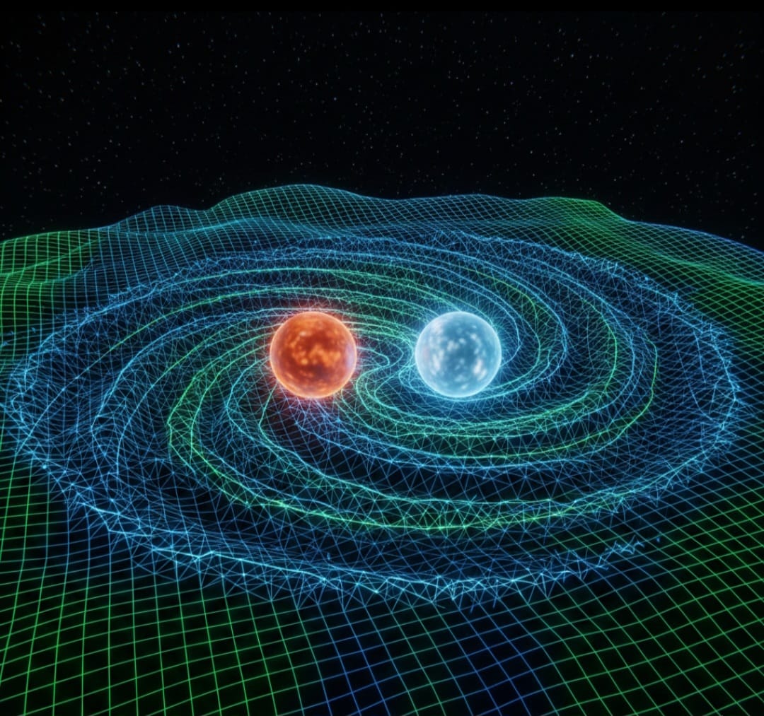
As we noted in the previous article in our series, Lorentz transformations use four variables to describe an event. Three of these are spatial dimensions and one is the time dimension. In physics, spacetime is defined as a four-dimensional mathematical model consisting of three spatial dimensions and one time dimension.

Spacetime Diagram

Spacetime diagrams are visual tools used to depict events in special relativity. With spacetime diagrams, phenomena such as time dilation and Lorentz contraction can be explained simply.

Any point in spacetime is called an event. The path followed by a particle forms a curve in spacetime. This curve is called the particle's worldline.

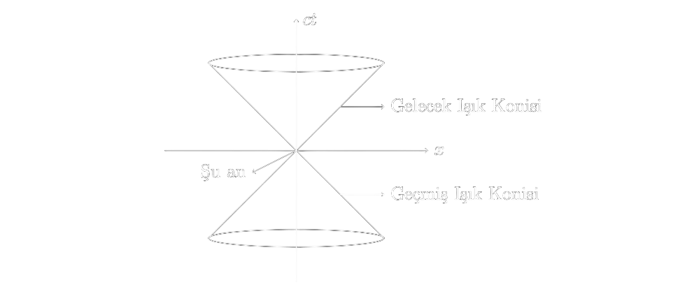
As shown in the figure, the future and past light cones of a particle can be seen. Within this cone lie the particle's possible future and past positions. An event occurring outside the cone cannot be observed by this particle. The boundaries of the cone are drawn at an angle of 45$^\circ$ because we take $c=1$. If we used the original value of $c$, the resulting figure would be very difficult to draw on paper. Moreover, although the $x$ and $ct$ axes are marked in the figure, depth has been added to make it appear three-dimensional. Thus, the graph depicts the $(ct,x,y)$ space. It is impossible to depict the $(ct,x,y,z)$ space.

Spacetime Diagram of a Moving Reference Frame

Let us recall the hyperbolic form of the Lorentz transformation shown in the previous part.

$$\begin{pmatrix} ct'\\x'\\y'\\z' \end{pmatrix}=\begin{pmatrix} ct\cosh \theta -x \sinh \theta \\ -ct\sinh \theta +x\cosh \theta \\ y\\ z \end{pmatrix}$$

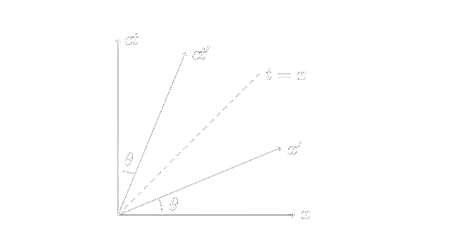
We will draw the spacetime diagram of the moving reference frame using the $ct'$ and $x'$ axes. To draw them, we must find the equations of the lines corresponding to these coordinates. To find the $ct'$ axis, let us set $x'=0$.

$$0=-ct\sinh \theta +x\cosh \theta$$ $$ct=x \coth \theta=x \left( \frac{c}{v}\right)$$

Similarly, to find the $x'$ axis, let us set $ct'=0$.

$$ct \cosh \theta- x \sinh \theta=0$$ $$ct=x \tanh \theta=x \left(\frac{v}{c}\right)$$

The lines drawn in this way give the spacetime diagram of the moving reference frame.

Spacetime Interval

An event is expressed using two different quantities: where the event occurs and when it occurs. An event can therefore be represented by three spatial coordinates and one time coordinate. Four-dimensional spaces with these properties are called Minkowski Spacetime.

In three-dimensional space, we express the distance $\Delta d$ between two points as

$$(\Delta d)^2=(\Delta x)^2+(\Delta y)^2+(\Delta z)^2$$

The distance $\Delta d$ remains the same regardless of the coordinate system we choose; in other words, $\Delta d$ is invariant. In four-dimensional spaces, the concept of an interval is defined by analogy with distance. Here, time is added as a fourth dimension. We combine space and time in this way because the two quantities are not invariant when considered separately. The time measured between two events by different observers will not be the same because of time dilation, nor will the distance between two events because of length contraction. By combining these two concepts, special relativity constructs an invariant that we call the spacetime interval. Consequently, all observers who measure the distance and time between two events obtain the same value from their calculations.
In four-dimensional Minkowski spacetime, the interval is defined as follows:

$$(\Delta s)^2 = -(c\Delta t)^2+(\Delta x)^2+(\Delta y)^2+(\Delta z)^2$$

If two events are infinitesimally close to each other, the interval $ds$ can also be written as

$$ds^2=-c^2dt^2+dx^2+dy^2+dz^2$$

When defining this spacetime interval, we stated that it is invariant. Let us now show explicitly why this is so. Let $ds^2$ denote the spacetime interval between two events as measured by an observer in frame $S$, and let ${ds'}^2$ denote the interval measured by the observer in $S'$. Since ${ds}^2$ and ${ds'}^2$ are related quantities, let us expand ${ds'}^2$ in a Taylor series.

$$ds'^2=\alpha+\beta ds^2+\gamma (ds^2)^2+ \dotsb$$

Let us neglect $(ds^2)^2$ and the subsequent terms because they are very small. To find $\alpha$, consider the case in which $ds^2=0$.

In this case,

$$ds^2=-c^2dt^2+dx^2+dy^2+dz^2=0$$ $$c^2dt^2=dx^2+dy^2+dz^2$$

This describes the path travelled by light in frame $S$. Since the speed of light is the same for all observers, we may write

$$c^2=\frac{dx^2+dy^2+dz^2}{dt^2}=\frac{{dx'}^2+{dy'}^2+{dz'}^2}{{dt'}^2}$$

As can be seen, if $ds=0$, then $ds'=0$ as well. From this, we find $\alpha=0$. The relation between $ds$ and $ds'$ therefore becomes

$$ds'^2=\beta ds^2$$

The coefficient $\beta$ here can depend only on the magnitude of the relative velocity between the two reference frames. It cannot depend on a coordinate or on time. If this coefficient depended on a coordinate or on time, we would obtain different values of $\beta$ at different temporal or spatial coordinates. That would contradict the homogeneous structure of spacetime. Likewise, because dependence on the direction of the relative velocity would contradict the isotropy of space, $\beta$ cannot depend on that direction. Therefore, the coefficient $\beta$ must depend on the magnitude of the relative velocity between the two reference frames.

Now let us consider three reference frames, $S$, $S_1$, and $S_2$. Let the velocities of $S_1$ and $S_2$ relative to $S$ be $V_1$ and $V_2$, respectively. Using the results we have found, we can write

$$ds^2=\beta(V_1){ds_1}^2\ \ \ \text{ve}\ \ \ ds^2=\beta(V_2){ds_2}^2$$

Let us also write the corresponding relation for $S_1$ and $S_2$:

$$ds_{1}^{2}=\beta(V_{12})ds_{2}^{2}$$ $$\beta(V_{12})=\frac{{ds_1}^2}{{ds_2}^2}=\frac{\beta(V_2)}{\beta(V_1)}$$

The problem here, however, is that $V_{12}$ depends not only on the velocities $V_1$ and $V_2$ but also on the angle between these two coordinate systems. This angle does not appear on the right-hand side of the equation. The only way for this equality to hold is for it to be equal to a constant, and that constant can only be one.

Thus,

$$ds^2={ds'}^2$$

may be written.

The Mathematics of Spacetime

From this point onward, we will denote spacetime coordinates using index notation. Each coordinate is numbered from 0 to 3, with the zeroth coordinate representing time.

$$x^{\mu}: \begin{pmatrix} x^0=ct\\x^1=x\\x^2=y\\x^3=z \end{pmatrix}$$

The superscripts here must not be interpreted as powers. Index notation allows us to write the spacetime interval more compactly. To do this, let us first define the \textit{Minkowski metric}. The components of the Minkowski metric are defined in a 4x4 matrix as follows:

$$\eta _{\mu \nu }= \begin{pmatrix} -1&0&0&0\\ 0&1&0&0\\ 0&0&1&0\\ 0&0&0&1 \end{pmatrix}$$

We will discuss what the concept of a metric means later; for now, this information is sufficient to develop what we have learned. Using this metric, we can write our spacetime interval as

$$ds^2= \sum_{\mu=0}^{3}\sum_{\nu=0}^{3}\eta_{\mu \nu}dx^{\mu}dx^{\nu}$$

Let us show that this does indeed correspond to the spacetime interval we defined. First, let us sum over the $\nu$ variables.

$$ds^2=\sum_{\mu=0}^{3}\left(\eta_{\mu 0}dx^{\mu}dx^{0}+\eta_{\mu 0}dx^{\mu}dx^{1}+\eta_{\mu 0}dx^{\mu}dx^{2}+\eta_{\mu 0}dx^{\mu}dx^{3}\right)$$ $$ds^2=\eta_{00}dx^0dx^0+\eta_{10}dx^1dx^0+\eta_{20}dx^2dx^0+\eta_{30}dx^3dx^0+\eta_{01}dx^0dx^1+\eta_{11}dx^1dx^1+\eta_{21}dx^2dx^1 \\ +\eta_{31}dx^3dx^1+\eta_{02}dx^0dx^2+\eta_{12}dx^1dx^2+\eta_{22}dx^2dx^2+\eta_{32}dx^3dx^2 +\eta_{03}dx^0dx^3+\eta_{13}dx^1dx^3+ \\ \eta_{23}dx^2dx^3+\eta_{33}dx^3dx^3$$

To simplify this calculation, recall that the matrix $\eta$ is diagonal. All $\eta_{\mu \nu}$ outside the diagonal ($\mu \neq \nu$) are equal to zero.

$$ds^2=\eta_{00}dx^0dx^0+\eta_{11}dx^1dx^1+\eta_{22}dx^2dx^2+\eta_{33}dx^3dx^3$$

Substituting the corresponding coordinate values in index notation gives

$$ds^2=-c^2dt^2+dx^2+dy^2+dz^2$$

which is the spacetime interval we defined. We can express this interval even more simply by dispensing with the summation symbols:

$$ds^2=\eta_{\mu \nu}dx^{\mu}dx^{\nu}$$

This is called the Einstein summation convention. According to this convention, repeated upper and lower indices are summed over all of their possible values. We can also write this expression in matrix form as

$$ds^2=(dx)^T \eta (dx)$$

Here, $(dx)^T$ is the transpose of the matrix $dx$.
Returning to the spacetime diagram, the definition of the interval shows that $ds^2$ can be less than, equal to, or greater than zero. For a point $p$ in the spacetime diagram, we can make the following statements:

$\bullet$ If $ds^2 <0$, point $p$ lies inside the light cone. In this case, any point inside the light cone is said to be timelike separated from point $p$.\
$\bullet$ If $ds^2=0$, point $p$ lies on the light cone. Any point on the light cone is said to be lightlike separated from point $p$.\
$\bullet$ If $ds^2>0$, point $p$ lies outside the light cone. Any point outside the light cone is said to be spacelike separated from point $p$.\
Now let us define proper time, an important concept in special relativity. Proper time is the time measured by the inertial reference frame moving along the path through spacetime. Like the interval, this quantity is invariant and is defined as

$$(d\tau)^2=-(ds)^2=-\eta_{\mu\nu}dx^{\mu}dx^{\nu}$$

Because the interval is negative for timelike-separated points, we define proper time by multiplying the interval by a minus sign.

Consider the rest frame $S$. Imagine a clock moving with velocity $v$ relative to $S$. Let us also introduce an inertial reference frame $S'$ that moves with the clock and has the clock at its origin. At any instant, an observer in $S$ measures the motion of the clock over the time interval $dt$ and measures the distance it travels during that time as $\sqrt{dx^2+dy^2+dz^2}$. The observer in $S'$ measures the clock's motion over the time interval $d\tau$ and measures it as travelling a distance $dx=dy=dz=0$, because the velocity of $S'$ relative to the clock is zero. Thus, writing the interval between the two events,

$$ds^2=-c^2dt^2+dx^2+dy^2+dz^2=-c^2{d\tau}^2+{dx'}^2+{dy'}^2+{dz'}^2=-c^2{d\tau}^2$$ $$\${d\tau}^2=\frac{-ds^2}{c^2}$$

Taking the square root of both sides,

$$d\tau=\frac{\sqrt{c^2dt^2-dx^2-dy^2-dz^2}}{c}=dt\left[1-\frac{1}{c^2}\left({\frac{dx}{dt}}\right)^2\right]^{1/2}=dt\sqrt{1-v^2/c^2}$$ $$d\tau=\gamma dt$$

we obtain the stated result.

We have reached the end of this part. In the next part, we will examine vectors, dual vectors, and tensors.