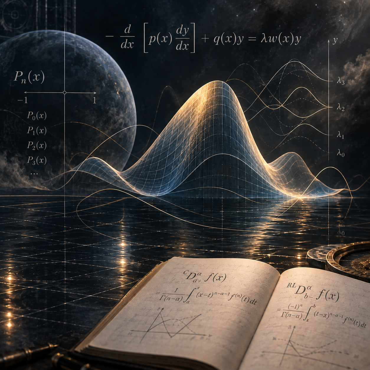
Fractional Sturm-Liouville Problems

Fractional Sturm–Liouville Problems

1. Introduction

Sturm–Liouville problems occupy a fundamental place in many areas of the natural sciences, engineering, and mathematics [1]. Although they were first formulated more than 170 years ago, they remain an active field of research and continue to be the subject of thousands of papers and books [1].

Let us first recall the basic structure of the classical Sturm–Liouville problem. A standard Sturm–Liouville differential equation is written as

$$-\frac{d}{dx}\left[p(x)\frac{dy}{dx}\right] + q(x)y = \lambda w(x)y$$

Here, $p(x)$, $q(x)$, and $w(x)$ are functions satisfying certain mathematical conditions. With a suitable transformation or integrating factor, many linear second-order differential equations can be brought into this general form. Important examples include the Hermite, Laguerre, Jacobi, and Legendre equations.

Now let us supplement the equation with appropriate boundary conditions. If $p(x)$ and $w(x)$ are positive throughout the interval and the relevant functions are continuous, the boundary conditions

$$\begin{aligned} c_{1}y(a) + c_{2}y'(a) &= 0, \quad (c_{1}^{2} + c_{2}^{2} > 0), \\ d_{1}y(b) + d_{2}y'(b) &= 0, \quad (d_{1}^{2} + d_{2}^{2} > 0), \end{aligned}$$

together with the equation define a regular Sturm–Liouville problem.

Two of the most important concepts here are eigenvalues and eigenfunctions. The values of $\lambda$ for which the equation and boundary conditions admit a nonzero solution are called eigenvalues, and the corresponding nonzero solutions are called eigenfunctions.

One of the fundamental results that makes Sturm–Liouville theory so powerful and useful is that, under suitable conditions, the eigenvalues are real and eigenfunctions corresponding to distinct eigenvalues are orthogonal with respect to a particular weight function. This property takes the theory beyond an abstract class of differential equations, making it useful in fields ranging from quantum mechanics to wave problems.

Not every problem is this regular. For example, if $p(x)$ vanishes at at least one endpoint of the interval, that is, at $x=a$ or $x=b$, the problem is called a singular Sturm–Liouville problem.

One of the most important examples of a singular problem is the Legendre differential equation. Frequently encountered in mathematical physics, this equation is written as

$$\frac{d}{dx}\left[(1-x^{2})\frac{dy}{dx}\right] + n(n+1)y = 0$$

Here, $p(x)=1-x^{2}$, so $p(x)$ vanishes at $x=-1$ and $x=1$. The Legendre problem is therefore a classic and important example of a singular Sturm–Liouville problem [2].

What we have discussed so far gives us the basic framework of classical Sturm–Liouville theory. But the really interesting part begins now.

The derivatives we have used so far have all had integer orders. What happens if we replace them with derivatives of fractional order? How does this affect the eigenvalues and eigenfunctions? Do the powerful properties of the classical theory survive in this new setting?

Before turning to these questions, let us briefly explore what fractional derivatives are, how they arose, and why they have become important in physics.

2. Preliminary Literature Review

What Are Fractional Derivatives, and How Did They Arise?

One of the most interesting exchanges in the history of mathematics took place in 1695 between Guillaume de l'Hôpital and Gottfried Wilhelm Leibniz. L'Hôpital asked Leibniz, one of the founders of differential calculus, a rather unusual question:

“What happens if the order $n$ of the derivative in $\frac{d^n y}{dx^n}$ is not an integer, but $n=1/2$?”

In other words, is it possible to take the half-order derivative of a function?

Leibniz's response is now regarded as one of the symbolic starting points in the development of fractional calculus:

“This is an apparent paradox, but one day very useful consequences will be drawn from it.”

Over time, Leibniz's prediction came true. In the centuries that followed, major mathematicians such as Euler, Laplace, Fourier, Liouville, Riemann, Letnikov, and Caputo pursued this question and helped establish the theoretical foundations of fractional calculus.

So what exactly is a fractional derivative?

Let us think about it in the simplest terms. If we can take the first and second derivatives of a function, why not its derivative of order one and a half, or of order $\pi$? Fractional calculus turns precisely this idea into a systematic mathematical theory.

The important point is that fractional differentiation involves more than simply “making the order of the derivative a fraction.” In many definitions of fractional derivatives, a function's past values are taken into account alongside its behavior at a given point. Fractional derivatives can therefore provide a mathematical description of how a system's past behavior affects its present state—in other words, its memory.

Whereas classical integer-order derivatives often describe a system's instantaneous rate of change, fractional derivatives can incorporate the contribution of past behavior to the present state. This makes fractional calculus a powerful tool for modeling systems influenced by their history, including damped vibrations, viscoelastic materials, signal transmission in the nervous system, and anomalous diffusion. Similar approaches are also used in certain systems, such as financial markets, where past behavior may be related to future movements [11, 12, 13, 14, 15].

Sturm–Liouville Theory and the Schrödinger Equation

To understand why fractional Sturm–Liouville problems matter, it is useful first to consider the place of classical Sturm–Liouville theory in mathematics and physics.

Sturm–Liouville theory is one of the fundamental mathematical frameworks for studying the eigenvalues and eigenfunctions of differential equations. To see how important this theory is to physics, we need only look at one of the central equations of quantum mechanics: the Schrödinger equation.

The time-independent, one-dimensional Schrödinger equation is written as

$$-\frac{\hbar^{2}}{2m} \frac{d^{2}\psi(x)}{dx^{2}} + V(x)\psi(x) = E\psi(x)$$

Here, $\hbar$ denotes the reduced Planck constant, $m$ the particle's mass, $V(x)$ the potential energy function, $E$ the particle's total energy, and $\psi(x)$ the wave function.

Now let us compare this equation with the classical Sturm–Liouville equation given in the introduction. At first glance, they may seem to be two equations with different physical meanings, but their mathematical structures are the same. With the appropriate identifications, the Schrödinger equation can be recast as a Sturm–Liouville problem.

This connection matters because the eigenvalues and eigenfunctions that arise in Sturm–Liouville theory correspond to physically meaningful quantities in quantum mechanics. In other words, when we study Sturm–Liouville theory, we are not dealing only with an abstract mathematical problem. We are also examining the mathematical structure that determines the energy levels of quantum systems and the states associated with them.

This is where fractional Sturm–Liouville problems come in. What mathematical structure emerges when we replace the derivatives in the classical Sturm–Liouville framework with fractional derivatives? How are the eigenvalues and eigenfunctions affected? More importantly, what properties does the new structure introduce that are absent from the classical theory?

These questions provide the central motivation for our study.

• $p(x) = \frac{\hbar^{2}}{2m}$ (A constant coefficient)
• $q(x) = V(x)$ (Potential energy)
• $w(x) = 1$ (Weight function)
• $y(x) = \psi(x)$ (Eigenfunctions: the probability amplitudes for finding the particle, that is, the wave function)
• $\lambda = E$ (Eigenvalues: the quantized energy levels available to the particle!)

One of the important results physicists encounter in quantum mechanics is the existence of discrete energy levels. Mathematically, these energies, written as $E_1, E_2, E_3, \ldots$, are simply the eigenvalues of Sturm–Liouville problems. Likewise, the orthogonality of wave functions corresponding to different energy states in quantum physics is a direct reflection of one of the fundamental results of Sturm–Liouville theory.

This is why studying fractional Sturm–Liouville problems means more than making an abstract mathematical generalization. When we consider a Sturm–Liouville problem involving fractional derivatives, we are also investigating how fractional derivatives may change the mathematical structure of quantum systems. This approach allows us to connect with more general physical models known as fractional quantum mechanics.

Of particular interest are systems that classical Brownian motion does not describe adequately, in which particles exhibit more complex motion than usual and past behavior affects the current dynamics. In such settings, where more general types of motion such as Lévy flights arise, fractional Schrödinger equations may be used in place of the classical Schrödinger equation.

Fractional Sturm–Liouville theory thus extends classical Sturm–Liouville theory to a more general mathematical framework while also allowing connections with physical models such as fractional quantum mechanics.

With this historical and physical background in place, let us now take a closer look at the basic tools of our study: fractional operators.

Essential Definitions and Theorems

Before turning to fractional Sturm–Liouville problems, let us recall some basic definitions of fractional integrals and derivatives that we will use in our study [25, 26]. These definitions are fundamental to understanding how the operators introduced in the following sections are constructed.

Fractional Integrals

First, let $\operatorname{Re}(\alpha)>0$. The left-sided and right-sided Riemann–Liouville fractional integrals of order $\alpha$ are defined, respectively, by

$$\begin{aligned} (I_{a^{+}}^{\alpha} f)(x) &= \frac{1}{\Gamma(\alpha)} \int_{a}^{x} (x-s)^{\alpha-1} f(s) \, ds, \quad x > a, \\ (I_{b^{-}}^{\alpha} f)(x) &= \frac{1}{\Gamma(\alpha)} \int_{x}^{b} (s-x)^{\alpha-1} f(s) \, ds, \quad x < b \end{aligned}$$

Here, $\Gamma$ is Euler's gamma function. In the left-sided integral, we proceed from $a$ to $x$, whereas in the right-sided integral, we proceed from $x$ to $b$. This two-sided structure will become one of the most important features of fractional Sturm–Liouville operators.

Fractional Derivatives

Now let us define fractional derivatives. Suppose that $\operatorname{Re}(\alpha)\in(m-1,m)$. The left-sided and right-sided Riemann–Liouville fractional derivatives of order $\alpha$ are then defined by

$$\begin{aligned} (D_{a^{+}}^{\alpha} f)(x) &= D^{m} (I_{a^{+}}^{m-\alpha} f)(x), \quad x > a, \\ (D_{b^{-}}^{\alpha} f)(x) &= (-D)^{m} (I_{b^{-}}^{m-\alpha} f)(x), \quad x < b \end{aligned}$$

By contrast, the left-sided and right-sided Caputo fractional derivatives of the same order are given by

$$\begin{aligned} ({}^{c}D_{a^{+}}^{\alpha} f)(x) &= (I_{a^{+}}^{m-\alpha} D^{m} f)(x), \quad x > a, \\ ({}^{c}D_{b^{-}}^{\alpha} f)(x) &= (I_{b^{-}}^{m-\alpha} (-D)^{m} f)(x), \quad x < b \end{aligned}$$

There is an important detail here: although the Riemann–Liouville and Caputo derivatives look very similar at first glance, the order in which differentiation and integration are performed is different. This distinction will be crucial to the structure of the fractional Sturm–Liouville operators we define later.

Integration by Parts in the Fractional Setting

The integration-by-parts formula familiar from calculus is a powerful tool for studying differential equations. A similar structure exists in fractional calculus. For our purposes, these formulas play an even more important role: we will construct the fractional Sturm–Liouville operators introduced shortly by drawing directly on these relations.

The relevant operators satisfy the following fractional integration-by-parts formulas:

$$\begin{aligned} \int_{a}^{b} f(x) I_{a^{+}}^{\alpha} g(x) \, dx &= \int_{a}^{b} g(x) I_{b^{-}}^{\alpha} f(x) \, dx, \\ \int_{a}^{b} f(x) D_{b^{-}}^{\alpha} g(x) \, dx &= \int_{a}^{b} g(x) {}^{c}D_{a^{+}}^{\alpha} f(x) \, dx + \sum_{k=0}^{m-1} (-1)^{m-k} f^{(k)}(x) D^{m-k-1} I_{b^{-}}^{m-\alpha} g(x)\Big|_{x=a}^{b}, \\ \int_{a}^{b} f(x) D_{a^{+}}^{\alpha} g(x) \, dx &= \int_{a}^{b} g(x) {}^{c}D_{b^{-}}^{\alpha} f(x) \, dx + \sum_{k=0}^{m-1} (-1)^{k} f^{(k)}(x) D^{m-k-1} I_{a^{+}}^{m-\alpha} g(x)\Big|_{x=a}^{b}. \end{aligned}$$

These formulas can be viewed as the fractional-calculus counterparts of classical integration by parts. They are particularly important because they show how left-sided and right-sided operators are related.

Composition Rules

We also need to know the relations that arise when fractional integrals and derivatives are applied successively. Let $\alpha\in(m-1,m)$, $\beta>\alpha$, and $f\in C[a,b]$. The following composition rules hold for every $x\in[a,b]$:

$$\begin{aligned} D_{a^{+}}^{\alpha} I_{a^{+}}^{\alpha} f(x) &= f(x), \quad D_{b^{-}}^{\alpha} I_{b^{-}}^{\alpha} f(x) = f(x), \\ D_{a^{+}}^{\alpha} I_{a^{+}}^{\beta} f(x) &= I_{a^{+}}^{\beta-\alpha} f(x), \quad D_{b^{-}}^{\alpha} I_{b^{-}}^{\beta} f(x) = I_{b^{-}}^{\beta-\alpha} f(x), \\ {}^{c}D_{a^{+}}^{\alpha} I_{a^{+}}^{\alpha} f(x) &= f(x), \quad {}^{c}D_{b^{-}}^{\alpha} I_{b^{-}}^{\alpha} f(x) = f(x), \\ I_{a^{+}}^{\alpha} I_{a^{+}}^{\beta} &= I_{a^{+}}^{\alpha+\beta}, \quad I_{b^{-}}^{\alpha} I_{b^{-}}^{\beta} = I_{b^{-}}^{\alpha+\beta}. \end{aligned}$$

These relations help us understand the algebraic structure of fractional operations and considerably simplify the calculations in the following sections.

Fractional Sturm–Liouville Problems

We can now turn to our main subject.

In a classical Sturm–Liouville problem, the structure of the differential operator determines important properties of the eigenvalues and eigenfunctions. We would like to extend this structure using fractional derivatives. But there is an important point here: we do not insert left-sided and right-sided fractional derivatives into the operator arbitrarily. We construct the new operator using the fractional integration-by-parts formulas we have just seen.

This approach is consistent with the central idea of classical Sturm–Liouville theory. In the classical theory, many important results concerning eigenvalues and eigenfunctions follow from integration by parts and the associated symmetry properties. Establishing a similar structure in the fractional case is therefore a natural starting point.

The Regular Fractional Sturm–Liouville Problem: Type I

Let us first define our fractional Sturm–Liouville operator as

$$\mathcal{L}_{\alpha,x} := {}^{c}D_{b^{-}}^{\alpha} p(x) D_{a^{+}}^{\alpha} + q(x)$$

The corresponding type I fractional Sturm–Liouville equation is

$$\mathcal{L}_{\alpha,x} f_{\lambda}(x) + \lambda w_{\alpha}(x) f_{\lambda}(x) = 0$$

Here, we assume that $p(x)\neq 0$ and $w_{\alpha}(x)>0$.

When the derivative order satisfies $0<\alpha<1$, our boundary conditions are

$$\begin{aligned} c_{1} I_{a^{+}}^{1-\alpha} f_{\lambda}(a) + c_{2} D_{a^{+}}^{\alpha} f_{\lambda}(a) &= 0, \\ d_{1} I_{a^{+}}^{1-\alpha} f_{\lambda}(b) + d_{2} D_{a^{+}}^{\alpha} f_{\lambda}(b) &= 0 \end{aligned}$$

For derivative orders $1<\alpha<2$, more boundary conditions are needed. In this case,

$$\begin{aligned} c_{1,0} I_{a^{+}}^{2-\alpha} f_{\lambda}(a) + c_{2,0} D p(x) D_{a^{+}}^{\alpha} f_{\lambda}(a)\Big|_{x=a} &= 0, \\ d_{1,0} I_{a^{+}}^{2-\alpha} f_{\lambda}(b) + d_{2,0} D p(x) D_{a^{+}}^{\alpha} f_{\lambda}(b)\Big|_{x=b} &= 0, \\ c_{1,1} D_{a^{+}}^{\alpha-1} f_{\lambda}(a) + c_{2,1} D_{a^{+}}^{\alpha} f_{\lambda}(a) &= 0, \\ d_{1,1} D_{a^{+}}^{\alpha-1} f_{\lambda}(b) + d_{2,1} D_{a^{+}}^{\alpha} f_{\lambda}(b) &= 0. \end{aligned}$$

We call the problem defined in this way a regular type I fractional Sturm–Liouville eigenvalue problem.

What Happens in the Singular Case?

Now consider the same differential equation:

$$\mathcal{L}_{\alpha,x} f_{\lambda}(x) + \lambda w_{\alpha}(x) f_{\lambda}(x) = 0.$$

This time, the difference lies in the behavior of $p(x)$ at the boundary points.

For $0<\alpha<1$, we assume

$$p(a)=p(b)=0$$

and for $1<\alpha<2$, we assume

$$p(a)=p(b)=0, \qquad p'(a)=p'(b)=0$$

The resulting problem is called a singular type I fractional Sturm–Liouville problem.

Here we see an important parallel with the classical theory: in the fractional case too, the distinction between regular and singular Sturm–Liouville problems is largely determined by the operator's behavior at the boundary points. With the introduction of fractional derivatives, however, both the operator's structure and the boundary conditions become quite different from those of the classical case.

Next, we will examine one of the most important aspects of these new problems: the behavior of their eigenvalues and eigenfunctions. In particular, tracing how the classical results on real eigenvalues and orthogonality arise in the fractional case leads to some interesting conclusions.

Are the Eigenvalues Real? Is Orthogonality Preserved?

We now come to two of the most important questions: are the eigenvalues of fractional Sturm–Liouville problems still real? Are eigenfunctions corresponding to distinct eigenvalues still orthogonal?

Much of the power of classical Sturm–Liouville theory comes from precisely these two properties. To see whether similar results hold in the fractional case, we will use the fractional integration-by-parts formulas introduced above.

Reality of the Eigenvalues

Our first theorem shows that an important property of the classical theory is preserved in the fractional setting:

[!theorem] Theorem 2.1
The eigenvalues of the regular type I fractional Sturm–Liouville problem are real.

To see this, suppose that there is an eigenfunction $y$ with a corresponding eigenvalue $\lambda$. Our equation is

$$\mathcal{L}_{\alpha,x} y(x) + \lambda w_{\alpha}(x)y(x) = 0$$

Using integration by parts to compare the operator's action on two functions gives

$$\int_{a}^{b} f(x) \mathcal{L}_{\alpha,x} g(x) \, dx = \int_{a}^{b} q(x)f(x)g(x) \, dx + \int_{a}^{b}p(x)D_{a^{+}}^{\alpha}f(x)D_{a^{+}}^{\alpha}g(x) \, dx + p(x)I_{a^{+}}^{1-\alpha}f(x)D_{a^{+}}^{\alpha}g(x)\Big|_{x=a}^{x=b}$$

Now let us write down and compare the eigenvalue equations for $y$ and its complex conjugate $\overline{y}$. Subtracting these equations in the appropriate way and integrating over $[a,b]$, we obtain

$$\begin{aligned} (\lambda-\overline{\lambda}) \int_{a}^{b}w_{\alpha}(x)|y(x)|^{2} \, dx &= p(b)\left[ I_{a^{+}}^{1-\alpha}y(b)D_{a^{+}}^{\alpha}\overline{y}(b) - I_{a^{+}}^{1-\alpha}\overline{y}(b)D_{a^{+}}^{\alpha}y(b) \right] \\ &\quad - p(a)\left[ I_{a^{+}}^{1-\alpha}y(a)D_{a^{+}}^{\alpha}\overline{y}(a) - I_{a^{+}}^{1-\alpha}\overline{y}(a)D_{a^{+}}^{\alpha}y(a) \right] \end{aligned}$$

This is where the boundary conditions come in. They eliminate the terms on the right-hand side, leaving

$$(\lambda-\overline{\lambda}) \int_{a}^{b}w_{\alpha}(x)|y(x)|^{2} \, dx = 0$$

Since $y$ is a nonzero eigenfunction and $w_{\alpha}(x)>0$, the integral is positive. Only one possibility remains:

$$\lambda = \overline{\lambda}.$$

In other words, the eigenvalues are real.

A similar argument gives this result for derivative orders in the interval $1<\alpha<2$. The boundary terms are somewhat more complicated in this case, but the appropriate boundary conditions again make all of them vanish. We also obtain the same conclusion for the singular problem:

[!theorem] Theorem 2.2
The eigenvalues of the singular type I fractional Sturm–Liouville problem considered in the space $C^{1+[\alpha]}[a,b]$ are real.

Introducing fractional derivatives into the equation therefore does not destroy this fundamental property of Sturm–Liouville theory.

Are the Eigenfunctions Still Orthogonal?

Now let us turn to the second fundamental property. In classical Sturm–Liouville problems, eigenfunctions corresponding to distinct eigenvalues are orthogonal. We can ask whether this remains true in the fractional case.

Once again, the answer is yes:

[!theorem] Theorem 2.3
Eigenfunctions of the regular type I fractional Sturm–Liouville problem corresponding to distinct eigenvalues are orthogonal with respect to the weight function $w_{\alpha}$. That is, if $\lambda_{1}\neq\lambda_{2}$, then

$$\int_{a}^{b} w_{\alpha}(x) f_{\lambda_{1}}(x) f_{\lambda_{2}}(x) \, dx = 0$$

The main idea of the proof is very similar to the method we just used to show that the eigenvalues are real.

Consider eigenfunctions $f_{\lambda_{1}}$ and $f_{\lambda_{2}}$ corresponding to two distinct eigenvalues, $\lambda_{1}$ and $\lambda_{2}$. Both functions solve the same fractional Sturm–Liouville equation, but for different eigenvalues.

Multiplying each equation by the other eigenfunction, subtracting, and then applying fractional integration by parts, we obtain

$$(\lambda_{1}-\lambda_{2}) \int_{a}^{b} w_{\alpha}(x) f_{\lambda_{1}}(x) f_{\lambda_{2}}(x) \, dx = p(b)[\cdots] - p(a)[\cdots]$$

The boundary conditions again eliminate the terms on the right-hand side. Thus,

$$(\lambda_{1}-\lambda_{2}) \int_{a}^{b} w_{\alpha}(x) f_{\lambda_{1}}(x) f_{\lambda_{2}}(x) \, dx = 0$$

Since $\lambda_{1}\neq\lambda_{2}$, this leaves

$$\int_{a}^{b} w_{\alpha}(x) f_{\lambda_{1}}(x) f_{\lambda_{2}}(x) \, dx = 0$$

Thus, eigenfunctions corresponding to distinct eigenvalues are orthogonal with respect to the weight function, just as in the classical theory.

The same result holds for the singular type I fractional Sturm–Liouville problem:

[!theorem] Theorem 2.4
Eigenfunctions of the singular type I fractional Sturm–Liouville problem corresponding to distinct eigenvalues are orthogonal with respect to the weight function. That is, if $\lambda_{1}\neq\lambda_{2}$, then

$$\int_{a}^{b} w_{\alpha}(x) f_{\lambda_{1}}(x) f_{\lambda_{2}}(x) \, dx = 0$$

An important result emerges here: even though we are using fractional derivatives, the two cornerstones of Sturm–Liouville theory—real eigenvalues and orthogonal eigenfunctions—survive under suitable conditions.

Moreover, when $q(x)=0$, we obtain an even more interesting orthogonality relation:

$$\int_{a}^{b} p(x) D_{a^{+}}^{\alpha}f_{\lambda_{1}}(x) D_{a^{+}}^{\alpha}f_{\lambda_{2}}(x) \, dx = 0.$$

This result opens up an important possibility for constructing new families of functions defined through fractional derivatives.

From Type I to Type II: Reflection

Let us now examine another interesting property of our operator. The type I operator we have defined does not map directly to itself under reflection. To study this, let us define a reflection operator by

$$\begin{aligned} Qf(x) &:= f(a+b-x), \\ Q^{2}f(x) &= f(x) \end{aligned}$$

This operator interchanges left-sided and right-sided fractional derivatives:

$$\begin{aligned} Q D_{a^{+}}^{\alpha} &= D_{b^{-}}^{\alpha}Q, \\ Q {}^{c}D_{a^{+}}^{\alpha} &= {}^{c}D_{b^{-}}^{\alpha}Q. \end{aligned}$$

We can therefore obtain a new fractional Sturm–Liouville operator by reflecting the type I operator:

$$\widetilde{\mathcal{L}}_{\alpha,x} := {}^{c}D_{a^{+}}^{\alpha} p(x) D_{b^{-}}^{\alpha} + q(x).$$

We may call the corresponding problem a type II fractional Sturm–Liouville problem.

The useful point here is that, if we know the solution of the type I problem, we can also obtain the solution of the type II problem by reflection.

[!proposition] Proposition 2.1
Any eigenfunction $f_{\lambda}$ of the regular type I fractional Sturm–Liouville problem, when reflected as $Qf_{\lambda}$, yields a solution of the type II fractional Sturm–Liouville problem.

This structure also shows that we can construct more general models. For example, a type III fractional Sturm–Liouville problem can be defined in which left-sided and right-sided fractional derivatives appear together in a more symmetric form. This more general structure, however, is a research topic in its own right.

The Fractional Legendre Equation

We now come to what may be the most surprising part of our study: the fractional Legendre equation.

Let us begin with Rodrigues' formula, which underlies the classical Legendre polynomials:

$$L_{n}(x) = \frac{(-1)^{n}}{2^{n}n!} D^{n}(1-x^{2})^{n} = \frac{(-1)^{n}}{2^{n}n!} D^{n}(1-x)^{n}(1+x)^{n}.$$

Here, the derivative order is an integer. We would like to carry the same idea into the fractional setting. To do so, we replace the classical derivatives with left-sided Riemann–Liouville and right-sided Caputo fractional derivatives.

The resulting equation is

$$\left[ {}^{c}D_{1^{-}}^{\alpha} (1-x^{2})^{\alpha} D_{-1^{+}}^{\alpha} + e_{2} \right]f(x) = 0$$

We call this the fractional Legendre equation.

A natural question arises at this point: what happens to the classical Legendre polynomials when we replace the derivatives in the classical Legendre equation with fractional derivatives?

This is where one of the most striking results of the study emerges. Although the new equation has a different eigenvalue structure from the classical equation, under suitable conditions it yields the same Legendre polynomials as eigenfunctions.

To understand this result, let us first examine the symmetry of the fractional operator. Applying fractional integration by parts gives

$$\int_{-1}^{1} \left[ f(x) {}^{c}D_{1^{-}}^{\alpha} (1-x^{2})^{\alpha} D_{-1^{+}}^{\alpha}g(x) - g(x) {}^{c}D_{1^{-}}^{\alpha} (1-x^{2})^{\alpha} D_{-1^{+}}^{\alpha}f(x) \right] dx = 0$$

This expression shows that the fractional Legendre operator is symmetric in the appropriate sense and provides the basis for studying the properties of its eigenfunctions.

Next, we will see the truly surprising result: why are the polynomials arising from the fractional Legendre equation the same as the classical Legendre polynomials, even though the eigenvalues change?

A Surprising Result: The Same Legendre Polynomials, Different Eigenvalues

We have finally reached one of the most surprising results of the study.

In deriving the fractional Legendre equation from the classical Legendre equation, we replaced the derivatives with fractional derivatives. At first glance, we might expect such a change to completely alter the solutions, particularly the Legendre polynomials. But that is not quite what happens.

[!theorem] Theorem 2.5
The classical Legendre polynomials $L_n(x)$ are also solutions of the following fractional Sturm–Liouville problem for every $\alpha>0$:

$$\left[ {}^{c}D_{1^{-}}^{\alpha} (1-x^{2})^{\alpha} D_{-1^{+}}^{\alpha} + e_{2}(\alpha,n) \right]L_n(x) = 0.$$

The eigenvalues, however, differ from those of the classical case and are given by

$$e_{2}(\alpha,n) = -\frac{\Gamma(n+1+\alpha)}{\Gamma(n+1-\alpha)}$$

The result is striking: we introduce fractional derivatives into the equation, yet the Legendre polynomials remain unchanged. It is the eigenvalues that change.

Let us briefly see how we obtain this result.

How Does This Result Emerge?

The proof begins by expressing the Legendre polynomials in powers of $(1+x)$ and then applying the left-sided Riemann–Liouville fractional derivative. Using the polynomial expansion gives

$$(1+x)^{\alpha}D_{-1^{+}}^{\alpha}L_n(x) = \sum_{j=0}^{n} a_j \frac{\Gamma(j+1)}{\Gamma(j+1-\alpha)} (1+x)^j$$

We then apply the right-sided Caputo fractional derivative to this expression. Rearranging the resulting terms as power series allows us to determine the coefficients of the fractional Legendre equation.

Solving the relations between these coefficients gives the eigenvalue directly as

$$e_{2}(\alpha,n) = -\frac{\Gamma(n+1+\alpha)}{\Gamma(n+1-\alpha)}$$

Here we can clearly see the difference from the classical Legendre equation. In the classical case, the eigenvalue has the form $n(n+1)$, whereas in the fractional case it becomes the gamma-function expression

$$-\frac{\Gamma(n+1+\alpha)}{\Gamma(n+1-\alpha)}$$

The fractional generalization thus changes the problem's eigenvalue structure while preserving its family of eigenfunctions.

Orthogonality Is Preserved Too

Another pleasing result is that these new solutions retain their orthogonality.

For distinct solutions of the fractional Legendre problem, we obtain

$$\int_{-1}^{1} L_{\alpha,n}(x)L_{\alpha,m}(x) \, dx = 0, \qquad n\neq m$$

The orthogonality of eigenfunctions corresponding to distinct eigenvalues was one of the most powerful features of Sturm–Liouville theory. The same structure appears here.

Moreover, using the linearity of the problem and mathematical induction, one can show that these fractional solutions are identical to the classical Legendre polynomials up to a constant factor.

We therefore have a rather unusual situation: We change the derivatives in the equation, and the eigenvalues change, but the eigenfunctions—the Legendre polynomials—stay the same.

New Orthogonal Functions from Fractional Derivatives

We can also use this structure of the Legendre polynomials to define new functions. For example, the functions defined by

$$P_n^{+}(x) := D_{-1^{+}}^{\alpha}L_n(x)$$

solve another fractional differential equation of their own:

$$\left[ D_{-1^{+}}^{\alpha} {}^{c}D_{1^{-}}^{\alpha} (1-x^{2})^{\alpha} + e_2(\alpha,n) \right]P_n^{+}(x) = 0.$$

These functions are also orthogonal with respect to the appropriate weight function:

$$\int_{-1}^{1} (1-x^{2})^{\alpha} P_n^{+}(x)P_j^{+}(x) \, dx = \frac{-e_2(\alpha,n)\delta_{n,j}}{n+\frac{1}{2}}.$$

Here, $\delta_{n,j}$ is the Kronecker delta, equal to one when $n=j$ and zero otherwise.

A similar structure is obtained for the functions $P_n^{-}$ defined using right-sided fractional derivatives.

These results show more than the existence of individual solutions. They also show that we can construct new systems of orthogonal functions through fractional derivatives.

Rewriting the Fractional Structure Using Legendre Series

Let us take these results a little further. Suppose that we expand two arbitrary functions in Legendre series. The integral of the product of their fractional derivatives can then be expressed in terms of the Legendre-series coefficients:

$$\begin{aligned} \int_{-1}^{1} (1-x^{2})^{\alpha} D_{-1^{+}}^{\alpha}f(x) D_{-1^{+}}^{\alpha}g(x) \, dx &= -\sum_{n=0}^{\infty} \frac{e_2(\alpha,n)a_nb_n}{n+\frac{1}{2}}, \\ \int_{-1}^{1} (1-x^{2})^{\alpha} D_{1^{-}}^{\alpha}f(x) D_{1^{-}}^{\alpha}g(x) \, dx &= -\sum_{n=0}^{\infty} \frac{e_2(\alpha,n)a_nb_n}{n+\frac{1}{2}}. \end{aligned}$$

These expressions allow us to study fractional differential operations through the coefficients of Legendre series. In other words, fractional differentiation that appears complicated can take on a much more orderly algebraic structure when we choose an appropriate function basis.

Finally, one can show that the functions $S_n^{+}$ and $S_n^{-}$ defined using fractional integrals also solve their corresponding fractional differential equations.

Starting from the Legendre polynomials, we thus obtain a broad family of related functions through fractional derivatives and integrals.

At this point, the theory has become quite powerful. But a natural question remains: do all these mathematical structures help us solve actual problems?

In the final part of the study, we pursue precisely this question and use the Legendre integral transform to solve two different fractional differential equations.

The Legendre Integral Transform

We now turn to an important tool that will put our theory to work: the Legendre integral transform.

The basic idea is simple. Instead of solving a complicated fractional differential equation directly, we move the problem to a new representation in terms of Legendre polynomials. This allows us to examine the differential operator's action through the coefficients in the function's Legendre series.

First, let us define an operator that we will use frequently in our study:

$$R_{\alpha} := {}^{c}D_{1^{-}}^{\alpha} (1-x^{2})^{\alpha} D_{-1^{+}}^{\alpha}$$

What Is the Legendre Integral Transform?

Suppose we want to represent a function $f(x)$ by a sequence of numbers rather than as a single function. This is exactly what the Legendre integral transform does.

[!definition] Definition 2.1
The Legendre integral transform maps the function $f(x)$ to the sequence of numbers $F(n)$ through the relation

$$F(n) = Tf := \int_{-1}^{1} f(x)L_n(x) \, dx$$

The Legendre series corresponding to the inverse transform is

$$T^{-1}F(n) = \sum_{n=0}^{\infty} \left(n+\frac{1}{2}\right) F(n)L_n(x)$$

The idea is much like that of the Fourier transform. Rather than working with a function directly, we expand it in a suitable family of functions—in this case, Legendre polynomials. Under appropriate conditions, this turns a continuous problem into a problem involving coefficients.

Let Us First Consider the Classical Case

Before moving to the fractional case, it is useful to examine the classical case $\alpha=1$.

In this case, the Legendre transform reduces the action of the operator $R_1$ to a very simple form:

$$TR_1f = n(n+1)F(n).$$

This result is meaningful because the classical Legendre polynomials are eigenfunctions of the relevant Sturm–Liouville operator. Applying the operator to a Legendre polynomial therefore simply gives a constant multiple of that polynomial.

Certain other integral operations can be expressed similarly under the Legendre transform:

$$TI_{1^{-}}^{1}(1+x)^{-1}f = \frac{(-1)^n}{2^n n!} \sum_{k=0}^{n} \left[ \sum_{j=k}^{n} a_n^j \frac{1}{j+1} c_j^k \right]F(k).$$

Here, $a_n^j$ and $c_j^k$ are coefficients obtained from the relevant expansions of the Legendre polynomials. Rather than giving their detailed expressions here, it is more useful to focus on the main idea behind the transform.

Moving to the Fractional Case

Now let us turn to the main question. What happens when we extend the structure obtained in the classical case to fractional derivatives?

The result takes a neat form:

[!proposition] Proposition 2.2
Under the Legendre integral transform, the fractional operator $R_{\alpha}$ acts as

$$TR_{\alpha}f = \frac{\Gamma(n+1+\alpha)}{\Gamma(n+1-\alpha)} F(n)$$

In addition, for fractional integrals,

$$\begin{aligned} TI_{1^{-}}^{\alpha}(1+x)^{-\alpha}f(x) &= \frac{(-1)^n}{2^n n!} \sum_{k=0}^{n} \left[ \sum_{j=k}^{n} a_n^j \frac{\Gamma(j+1)}{\Gamma(j+\alpha+1)} c_j^k \right]F(k), \\ TI_{-1^{+}}^{\alpha}(1-x)^{-\alpha}f(x) &= \frac{1}{2^n n!} \sum_{k=0}^{n} \left[ \sum_{j=k}^{n} a_n^j \frac{\Gamma(j+1)}{\Gamma(j+\alpha+1)} c_j^k(-1)^k \right]F(k). \end{aligned}$$

The first result is particularly important. Under the Legendre transform, the action of the fractional operator becomes multiplication by

$$\frac{\Gamma(n+1+\alpha)}{\Gamma(n+1-\alpha)}$$

rather than a complicated fractional differential operation.

This also explains why the fractional Legendre equation is so useful. The fractional differential operator, which looks quite complicated when considered directly in $x$-space, takes on a much simpler algebraic structure under the Legendre transform.

The proofs of these results rely primarily on the definition of the Legendre transform. The definition of the fractional integral is inserted into the transform integral, the Legendre polynomials are expanded, and the terms are rearranged. Lengthy calculations of the coefficients yield the expressions above. For the right-sided integral, the reflection symmetry of the Legendre polynomials is used.

In other words, the Legendre transform is more than an alternative representation here. It becomes one of our main tools for solving fractional differential equations.

In the next section, we will see the power of this transform directly. We will use the Legendre transform to solve two different fractional differential equations and show how the theory developed so far becomes a concrete method of solution.

Applications: Let Us Solve Actual Problems

We can now see the real value of the theory we have developed. We have defined fractional Sturm–Liouville operators, examined their basic properties, established the connection between Legendre polynomials and these new equations, and developed the Legendre integral transform.

Now let us use all these tools to solve actual differential equations.

Variational Problems

First, consider a more general equation that arises from a variational problem and contains a free parameter and an external forcing term. After fractional integration by parts, the problem becomes the nonhomogeneous fractional differential equation

$$[R_{\alpha}-\lambda]f(x) = g(x)$$

Here, $g(x)$ represents an externally applied influence, and $\lambda$ is the free parameter in the problem.

This is precisely where the power of the Legendre integral transform comes into play. Taking the transform of the equation turns the differential equation into a much simpler algebraic relation for the Legendre coefficients:

$$F(n) = -\frac{G(n)}{e_2(\alpha,n)+\lambda}.$$

Applying the inverse Legendre transform then gives the solution directly as a series:

$$f(x) = -\sum_{n=0}^{\infty} \left(n+\frac{1}{2}\right) \frac{G(n)}{e_2(\alpha,n)+\lambda} L_n(x).$$

This provides a clear example: a fractional differential equation that initially looks complicated becomes a simple problem that can be solved through its coefficients once an appropriate function basis is chosen.

The solution obtained here is a particular solution. To obtain the general solution, we must also add a solution of the homogeneous equation

$$[R_{\alpha}-\lambda]f_0(x) = 0$$

More Complicated Operators Are Possible Too

A useful feature of our method is that it is not limited to a single fractional operator. The same approach can be applied to operators with several components involving multiple fractional derivatives and integrals.

Although the resulting equations may look much more complicated, the basic idea remains the same: move the equation to Legendre space, determine the coefficients, and then apply the inverse transform. Under suitable convergence conditions, similar series solutions can be obtained for these more general operators as well.

Fractional Diffusion

Now let us turn to a more directly physical problem: diffusion.

The classical diffusion equation describes how matter or energy spreads through space over time. In some systems, however, this spreading departs from classical diffusion. Particularly when the history of the medium matters, fractional derivatives become a natural tool for modeling this behavior.

Let us therefore consider the following model, which is classical in the time variable and fractional in the spatial variable:

$$-k_{\alpha}R_{\alpha,x}u(x,t) = \frac{\partial u(x,t)}{\partial t}.$$

Let our initial condition be

$$u(x,0) = g(x)$$

Applying the Legendre integral transform again turns the fractional spatial operator into multiplication by an eigenvalue. The original partial differential equation thus separates into an independent ordinary differential equation for each Legendre coefficient.

The resulting solution is

$$u^{c}(x,t) = \sum_{n=0}^{\infty} \left(n+\frac{1}{2}\right) G(n) e^{k_{\alpha}e_2(\alpha,n)t} L_n(x)$$

Here, $G(n)$ denotes the Legendre-transform coefficients of the initial function.

The idea behind this formula is actually quite simple. Instead of solving the original complicated fractional partial differential equation directly, we first decompose it in terms of Legendre polynomials. We then only need to solve an ordinary differential equation for each component. Finally, we put all the components back together to obtain the solution $u(x,t)$.

Under suitable conditions, the series can also be shown to converge uniformly. We therefore obtain a mathematically well-defined solution, rather than merely a formal one.

This approach can be extended to include boundary value problems. By adding appropriate steady-state solutions, we can study the time-dependent solution together with the equilibrium state that emerges at long times.

Fractional Diffusion with Reflection Symmetry

As a next step, we can also take the reflection symmetry of the diffusion operator into account.

If both the problem and the initial function have reflection symmetry, we can use the following properties of the Legendre polynomials:

$$L_{2n}(-x)=L_{2n}(x), \qquad L_{2n+1}(-x)=-L_{2n+1}(x)$$

When the initial function is even, the odd-indexed Legendre coefficients vanish automatically. The solution then consists only of Legendre polynomials of even degree.

In this case, the series solution simplifies considerably:

$$u(x,t) = \sum_{n=0}^{\infty} \left(2n+\frac{1}{2}\right) G(2n) e^{k_{\alpha}e_2(\alpha,2n)t} L_{2n}(x).$$

This result shows how the symmetry of the problem is directly reflected in the mathematical structure of its solution.

The method remains the same if a $\lambda$ term is added to the model. The corresponding parameter is simply included in the exponential describing the time dependence. This yields a more general symmetric fractional diffusion model.

Where Can We Go from Here?

The method described here is not limited to Legendre polynomials.

The same approach can be applied to other classical Sturm–Liouville systems, such as the Laguerre or Jacobi equations. Using the integral transform associated with each family of functions may allow us to obtain new fractional operators and new classes of differential equations.

Similarly, combining different Legendre transforms or using more general fractional derivatives in place of the classical Riemann–Liouville derivatives may open up new lines of research. The different definitions of fractional derivatives in the literature offer considerable scope for developing such new Sturm–Liouville models.

The theory presented here can therefore be seen less as a finished story than as a starting point leading to new problems.

Conclusion

We have now reached the end of our journey.

We first saw why classical Sturm–Liouville theory is one of the fundamental tools of mathematics and physics. We then went beyond classical derivatives to define new fractional Sturm–Liouville operators combining left-sided and right-sided Riemann–Liouville and Caputo fractional derivatives.

We showed that these new problems are more than formal generalizations. We established that the eigenvalues of regular and singular problems are real and that eigenfunctions corresponding to distinct eigenvalues remain orthogonal with respect to the appropriate weight function.

We then examined the fractional Legendre equation and obtained what may be the study's most surprising result: the classical Legendre polynomials also appear as solutions of the fractional Legendre equation. The eigenvalues, however, change and are expressed through gamma functions as

$$e_2(\alpha,n) = -\frac{\Gamma(n+1+\alpha)}{\Gamma(n+1-\alpha)}$$

We subsequently used the Legendre integral transform to apply this theory to concrete problems. We obtained series solutions for nonhomogeneous fractional differential equations arising from a variational formulation and analytically solved diffusion equations involving fractional derivatives in the spatial variable. We also showed that, under suitable conditions, the resulting series converge uniformly.

These results show that fractional Sturm–Liouville theory is not merely an abstract mathematical structure. It is a powerful tool for modeling and solving problems such as diffusion and more general fractional differential equations.

Perhaps the most exciting point is that what we have done here represents only a small part of fractional Sturm–Liouville theory. We do not yet fully know what will happen when we use other classical families of orthogonal polynomials in place of Legendre polynomials. Discovering which new operators and special functions arise from more general fractional derivatives, different integral transforms, and different symmetries remains an open area of research.

In short, there is still a great deal to explore in this new setting where classical Sturm–Liouville theory meets fractional calculus.

Appendix: Applying Rodrigues' Formula Step by Step

For readers wondering where the coefficients used in this section come from, let us examine Rodrigues' formula step by step.

With $D=d/dx$, the classical Legendre polynomials are defined by

$$L_n(x) = \frac{(-1)^n}{2^n n!} D^n(1-x^2)^n = \frac{(-1)^n}{2^n n!} D^n(1-x)^n(1+x)^n$$

First, let us write the polynomial in terms of $(1+x)^j$:

$$\begin{aligned} L_n(x) &= \frac{(-1)^n}{2^n n!} D^n \sum_{j=0}^{n} \binom{n}{j} 2^{n-j}(-1)^j (1+x)^{n+j} \\ &= \frac{(-1)^n}{2^n n!} \sum_{j=0}^{n} \binom{n}{j} 2^{n-j}(-1)^j \frac{\Gamma(n+j+1)}{\Gamma(j+1)} (1+x)^j \\ &= \frac{(-1)^n}{2^n n!} \sum_{j=0}^{n} a_n^j(1+x)^j. \end{aligned}$$

By reflection, the same procedure can be carried out for terms of the form $(1-x)^j$:

$$L_n(x) = \frac{1}{2^n n!} \sum_{j=0}^{n} a_n^j(1-x)^j.$$

These expansions play a fundamental role when applying fractional integration to Legendre polynomials.

For example, applying the left-sided fractional integral gives

$$(1+x)^{-\alpha} I_{-1^{+}}^{\alpha}L_n(x) = \frac{(-1)^n}{2^n n!} \sum_{j=0}^{n} a_n^j \frac{\Gamma(j+1)}{\Gamma(j+\alpha+1)} (1+x)^j$$

In the final step, we express the terms $(1+x)^j$ in terms of Legendre polynomials again. The coefficients are

$$\begin{aligned} c_j^m &= \left(m+\frac12\right) \int_{-1}^{1} L_m(x)(1+x)^j \, dx \\ &= \left(m+\frac12\right) \frac{(-1)^m}{2^m m!} \sum_{l=0}^{m} a_m^l \frac{2^{l+j+1}}{l+j+1} \end{aligned}$$

Therefore,

$$(1+x)^j = \sum_{k=0}^{j} \left[ \left(k+\frac12\right) \frac{(-1)^k}{2^k k!} \sum_{l=0}^{k} a_k^l \frac{2^{l+j+1}}{l+j+1} \right] L_k(x).$$

The purpose of these calculations is more than simply to obtain coefficients. More importantly, they allow us to see clearly how Legendre polynomials behave under fractional integration and differentiation. This is precisely the algebraic structure behind the transform formulas obtained in the preceding sections.

References

1. A. Zettl, Sturm-Liouville Theory, Mathematical Surveys and Monographs, vol. 121, American Mathematical Society, 2005.
2. R. Courant, D. Hilbert, Methods of Mathematical Physics, Volume 1, Interscience Publishers, Inc., New York, 1953.
3. C.J. Tranter, Legendre transforms, Quart. J. Math. Oxford Ser. (2) 1 (1950) 1–8.
4. R.V. Churchill, New operational mathematics—the operational calculus of Legendre transforms, Technical Report No. 1, Project 2137 Ordnance Corps, US Army, Contract No. DA-20-018-ORD-12916, August, 1953.
5. L. Debnath, C.W. Harrell, The operational calculus of associated Legendre transforms-1, Indian J. Pure Appl. Math. 7 (1976) 278–291.
6. L. Debnath, D. Bhatta, Integral Transforms and their Applications, second ed., Chapman & Hall/CRC, Taylor & Francis Group, New York, 2007.
7. R.K. Gupta, S.D. Gupta, Operational calculus of spheroidal wave angle functions (generalized Legendre transform), Indian J. Pure Appl. Math. 8 (1976) 602–610.
8. R.K. Gupta, S.D. Gupta, Some operational properties of generalized Legendre transform and their applications II, Indian J. Pure Appl. Math. 8 (1976) 589–601.
9. P.L. Butzer, R.L. Stens, M. Wehrens, The continuous Legendre transform, its inverse transform, and applications, Int. J. Math. Math. Sci. 3 (1) (1980) 47–67.
10. E.Y. Deeba, E.L. Koh, Operational calculus for the continuous Legendre transform with applications, Int. J. Math. Math. Sci. 12 (2) (1989) 355–362.
11. A. Carpinteri, F. Mainardi (Eds.), Fractals and Fractional Calculus in Continuum Mechanics, Telos, Springer-Verlag, 1998.
12. R. Hilfer (Ed.), Applications of Fractional Calculus in Physics, World Scientific, Singapore, 2000.
13. R.L. Magin, Fractional Calculus in Bioengineering, Begell House Inc., Redding, CT, 2006.
14. I. Podlubny, Fractional Differential Equations, Academic Press, San Diego, CA, USA, 1999.
15. B.J. West, M. Bologna, P. Grigolini, Physics of Fractal Operators, Springer Verlag, New York, NY, 2003.
16. M. Klimek, O.P. Agrawal, On a regular fractional Sturm-Liouville problem with derivatives of order in (0,1), in: Proceedings of the 13th International Carpathian Control Conference, Vysoke Tatry (Podbanske), Slovakia, 28–31 May 2012. http://dx.doi.org/10.1109/CarpathianCC.2012.6228655.
17. Q.M. Al-Mdallal, An efficient method for solving fractional Sturm-Liouville problems, Chaos Solitons Fractals 40 (2009) 183–189.
18. Q.M. Al-Mdallal, On the numerical solution of fractional Sturm-Liouville problems, Int. J. Comput. Math. 87 (2010) 2837–2845.
19. A. Neamaty, R. Darzi, A. Dabbaghian, J. Golipoor, Introducing an iterative method for solving a special FDE, Int. Math. Forum 4 (2009) 1449–1456.
20. V.S. Erturk, Computing eigenelements of Sturm-Liouville problems of fractional order via fractional differential transform method, Math. Comput. Appl. 16 (2011) 712–720.
21. J. Qi, S. Chen, Eigenvalue problems of the model from nonlocal continuum mechanics, J. Math. Phys. 52 (073516) (2011).
22. T.M. Atanackovic, B. Stankovic, Generalized wave equation in nonlocal elasticity, Acta Mech. 208 (2009) 1–10.
23. M. d'Ovidio, From Sturm-Liouville problems to fractional and anomalous diffusions, Stochastic Process. Appl. 122 (2012) 3513–3544.
24. D. Baleanu, K. Diethelm, E. Scalas, Fractional Calculus: Models and Numerical Methods, World Scientific Publishing Company, Singapore, 2012.
25. A.A. Kilbas, H.M. Srivastava, J.J. Trujillo, Theory and Applications of Fractional Differential Equations, Elsevier, Amsterdam, Netherlands, 2006.
26. S.G. Samko, A.A. Kilbas, O.I. Marichev, Fractional Integrals and Derivatives: Theory and Applications, Gordon and Breach, PA, 1993.
27. D. Baleanu, J.A. Tenreiro Machado, A.C.J. Luo (Eds.), Fractional Dynamics and Control, Springer, New York, NY, 2012.
28. M. Klimek, On Solutions of a Linear Fractional Differential Equations of a Variational Type, The Publishing Office of the Czestochowa University of Technology, Czestochowa, 2009.
29. O.P. Agrawal, Generalized variational problems and Euler-Lagrange equations, Comput. Math. Appl. 59 (2010) 1852–1864.
30. O.P. Agrawal, Some generalized fractional calculus operators and their applications in integral equations, Fract. Calc. Appl. Anal. 15 (4) (2012) 700–711.
31. M. Klimek, O.P. Agrawal, Regular fractional Sturm-Liouville problem with generalized derivatives of order in (0,1), in: Proceedings of the IFAC Joint Conference: 5th SSSC, 11th WTDA, 5th WFDA, Grenoble, France, 4–6 February 2013 (in press).
32. J.L. Forman, M. Soerensen, The Pearson diffusions: a class of statistically tractable diffusion processes, Scand. J. Statist. 35 (2008) 438–465.
33. N.N. Leonenko, M.M. Meerschaert, A.A. Sikorskii, Fractional Pearson diffusion, 2011. Preprint http://www.stt.msu.edu/~mcubed/LMS.pdf.