Foundation of Quantum Mechanics 1

Foundations of Quantum Mechanics — 1

The Classical Physics Worldview Before Quantum Mechanics

Introduction: Why Start with Classical Physics?

This article is the first part of a series on the foundations of quantum mechanics. The main aim of the series is to go beyond the equations of quantum mechanics and examine how those equations explain the world. But before moving on to quantum mechanics, some preparation is necessary. First, it is important to lay out the classical-physics perspective clearly. Knowing the basic concepts, laws, and intuitions of classical physics plays a critical role in understanding where quantum mechanics challenges this framework and how it offers a new perspective. Seeing the points of continuity and rupture between classical and quantum physics makes it easier to understand the conceptual difficulties encountered in quantum-mechanical problems. Because “classical physics” and “quantum physics” will be compared continuously throughout the series, this first article is devoted entirely to establishing the classical framework. Quantum mechanics itself will begin only in the next article.

It is appropriate to begin with an attitude that is common in standard quantum-mechanics education:

Shut up and calculate.

The idea behind this approach is simple. The Schrödinger equation works in experiments and gives correct predictions. Therefore, there is no need to ask what the wave function “really is.” One takes the equation and performs the calculation. One says, “This outcome occurs with such-and-such probability.” And that is the end of the matter. What happens behind the curtain is left unexplored.

It must be acknowledged that this approach has been extremely successful in practice. But this series was written precisely to look behind that curtain. Because the following questions should not remain unanswered:

What is the wave function? What does its “collapse” mean? Can a particle really be in more than one place at the same time?

In the literature, this field is known as the Foundations of Quantum Mechanics. A significant part of the subject, however, is devoted to the interpretations of quantum mechanics. So a question should be asked at the very beginning: what exactly is meant by an “interpretation” — and what is the difference between an interpretation and a physical theory?

Interpretation or Physical Theory?

In the quantum-mechanics literature, the word “interpretation” is used very loosely. Examples include the Copenhagen interpretation, the pilot-wave interpretation, and the many-worlds interpretation. The philosopher of physics Tim Maudlin, however, objects to this usage. According to Maudlin, many of the things called “interpretations of quantum mechanics” are not really interpretations at all, but distinct physical theories (see Tim Maudlin, Philosophy of Physics: Quantum Theory, Princeton University Press, 2019).

Maudlin’s distinction is based on the following criterion. For a physical theory to count as complete, it must clearly specify three things:

1. Ontology: According to the theory, what exists in the world? Are there particles, fields, or perhaps the wave function itself?

2. Dynamics: How do these entities behave over time, and what laws do they obey?

3. Connection to measurement: How are the quantities in the theory related to the outcomes observed in the laboratory?

When these criteria are applied, the status of the candidates usually called “interpretations” changes as follows:

Candidate	Status according to Maudlin’s distinction
Pilot wave (Bohmian mechanics)	Proposes a different ontology: there are particles and a wave that guides them. It is a distinct physical theory.
Objective collapse (GRW)	Proposes different dynamics: it adds random collapses to Schrödinger evolution. Moreover, it produces predictions that are, in principle, different from standard quantum mechanics. It is a distinct physical theory.
Copenhagen	Provides neither a clear ontology nor a consistent dynamics; it says, in effect, “collapse occurs during measurement — do not ask for more.” According to Maudlin, this is not even a theory, but rather an attitude or a practical rulebook.
Many worlds	Because it keeps the same dynamics and attempts mainly to change the “story,” it is the candidate closest to being a genuine interpretation — although even this is debatable.

The status of the candidates according to Maudlin’s three criteria

A short example makes the distinction clearer. Bohm’s pilot-wave theory says that particles genuinely exist in the subatomic world (ontology), gives a precise law for how those particles move (dynamics), and provides a connection between the theory and measurement outcomes. By contrast, the standard Copenhagen interpretation does not clearly state what the wave function actually represents, does not specify what “really” happens during measurement, and remains ambiguous about ontology. In other words, Bohmian theory clearly satisfies Maudlin’s three criteria, whereas the Copenhagen approach functions more as a practical attitude. The importance of this distinction for the rest of the series is the following: in Maudlin’s framework, the question “Which interpretation of quantum mechanics is correct?” is really the question “Which physical theory about the world is correct?” The issue is therefore not a matter of wordplay or aesthetic preference; it is a matter of what exists, what laws govern it, and what the theory predicts. In later articles, each candidate will be evaluated according to these three criteria — what its ontology is, what its dynamics are, and how it connects to measurement.

Problems to Be Examined in the Series

Throughout the series, four main problem areas and the candidate theories that attempt to answer them will be examined.

The measurement problem: What is a measurement? What makes an interaction a “measurement”? What distinguishes a measurement from an interaction that is not a measurement? What exactly happens when a “classical” measuring device interacts with a “quantum” system? Must the world be divided into a quantum realm and a classical realm? These questions appear simple at first. Their answers are anything but simple.

Locality and causality: When one of two entangled particles is measured and the joint wave function of the pair collapses, it can look as if a message is sent to the distant particle: “A collapse happened here.” But does this message travel faster than light? There is another important point: this “message” cannot be used to send controlled information (the no-signaling principle). The question therefore becomes: what exactly does the speed-of-light limit forbid — every kind of influence at a distance, or only the transmission of usable information? This question leads directly to a reconsideration of the concept of causality itself.

Ontology: Ontology asks the question, “What exists?” The wave function is often described as a “probability wave.” But probability, in the classical sense, is not matter or a tangible “thing.” Quantum mechanics, however, seems almost to force us to consider the possibility that probability itself is something mind-independent and genuinely present in the world. The same question applies to fields and potentials. Is the electromagnetic field something that really exists? Are photons merely excitations of it? Or are these concepts only mathematical tools that make calculations easier?

Interpretations and candidate theories: Several candidates arise when we ask how the wave function and its collapse should be understood:

Candidate	Brief description
Copenhagen	The standard view. The wave function evolves according to the Schrödinger equation and collapses when a measurement is performed. What collapse “is” is not investigated; this is the approach most compatible with “shut up and calculate.” (By Maudlin’s criteria, it is not a theory but an attitude; see Section 2.)
Pilot wave	The wave is something real and guides the particle like a pilot; the particle is carried along under the guidance of the wave.
Objective collapse (GRW)	Collapse is an intrinsic feature of the wave function; it occurs spontaneously and randomly, without requiring an observer or a measurement. It incorporates into the dynamics the collapse that Copenhagen adds from outside the theory.
Many worlds	Every measurement divides the world into multiple branches (or worlds).

Candidate theories concerning the wave function and collapse

In addition, Bell’s theorem will be examined. It is especially important to emphasize that Bell’s theorem is not an interpretation: the theorem concerns nature itself, not any particular interpretation. Read together with the EPR argument, it produces a two-step line of reasoning. In the first step, the perfect correlations observed in entangled pairs imply — under the assumption of locality (technically, local causality) — that the particles must possess definite properties even before measurement, that is, hidden variables. In the second step, Bell proves that such local variables cannot reproduce the correlations predicted by quantum mechanics; experiments have confirmed the quantum predictions. The conclusion is therefore not, as is often said, that “hidden variables have been ruled out.” What has been ruled out is locality. A hidden-variable theory remains possible; it simply cannot be local — and pilot-wave theory is precisely such a theory.

Throughout the series, we will follow Travis Norsen’s Foundations of Quantum Mechanics: An Exploration of the Physical Meaning of Quantum Theory.

We can now turn to how the classical-physics worldview is constructed. This worldview has two main components: Newtonian mechanics and Maxwellian electrodynamics. Einstein’s special theory of relativity is also usually included.

The Newtonian Worldview

In the Newtonian picture, the universe obeys Newton’s three laws of motion at every level, from the largest cosmic scales down to the smallest scales.

Fundamental Structure and Atomism

In Newtonian mechanics, the physical universe consists of hard, massive, unbreakable, and indivisible microscopic particles that move and interact with one another through forces. This assumption forms a bridge between ancient Greek atomism and the modern chemical/physical atomic theory.

In this picture, the universe’s “list of ingredients” contains only two items: particles and the forces that those particles exert on one another. Everything in the visible world — rocks, water, air, living organisms — is nothing more than an arrangement of tiny and indestructible particles too small to be seen with the naked eye. The three laws of motion listed below govern the behavior of each of these fundamental particles.

Deriving Macroscopic Laws

The fact that macroscopic bodies (planets, apples, and so on) obey Newton’s laws is not a fundamental axiom, but a theorem derived from the fundamental laws governing microscopic particles.

This subtlety is important. The fall of an apple from a tree and the orbit of the Moon are not separate and independent laws of nature. A macroscopic body is the sum of countless particles; if each particle obeys the fundamental laws, the behavior of the whole can be calculated, and the result reproduces exactly the macroscopic laws we observe. In other words, the order seen at large scales is a derived consequence of the laws at small scales. This “bottom-up” form of explanation will become the template for much of later physics: for a theory to count as “fundamental,” we expect it to be able to derive the familiar laws of the everyday world from its own fundamental ingredients. The same criterion will be used in later articles when evaluating candidate theories of quantum mechanics.

First Law: Inertia

A body remains at rest, or continues to move in a straight line at constant velocity, unless a net external force acts on it.

This is the law of inertia. An external force is required to change the state of motion of a body. If no force acts, the velocity vector — both its magnitude and its direction — remains constant.

Second Law: Force and Momentum

When a force acts on a body, the rate of change of its momentum with respect to time is equal to the applied force:

$$\mathbf{F} = \frac{d\mathbf{p}}{dt}$$

Momentum is defined as the product of mass and velocity:

$$\mathbf{p} = m\mathbf{v}$$

When the mass is constant, applying the chain rule gives the familiar form:

$$\mathbf{F} = \frac{d}{dt}(m\mathbf{v}) = m\frac{d\mathbf{v}}{dt} = m\mathbf{a}$$

If more than one force acts on a body, what matters is their vector sum:

$$\mathbf{F}_{\text{net}} = \sum_{i} \mathbf{F}_i = m\mathbf{a}$$

The meaning of this is illustrated in the diagram below. Suppose a large force acts on an object to the right, while two smaller forces act to the left:

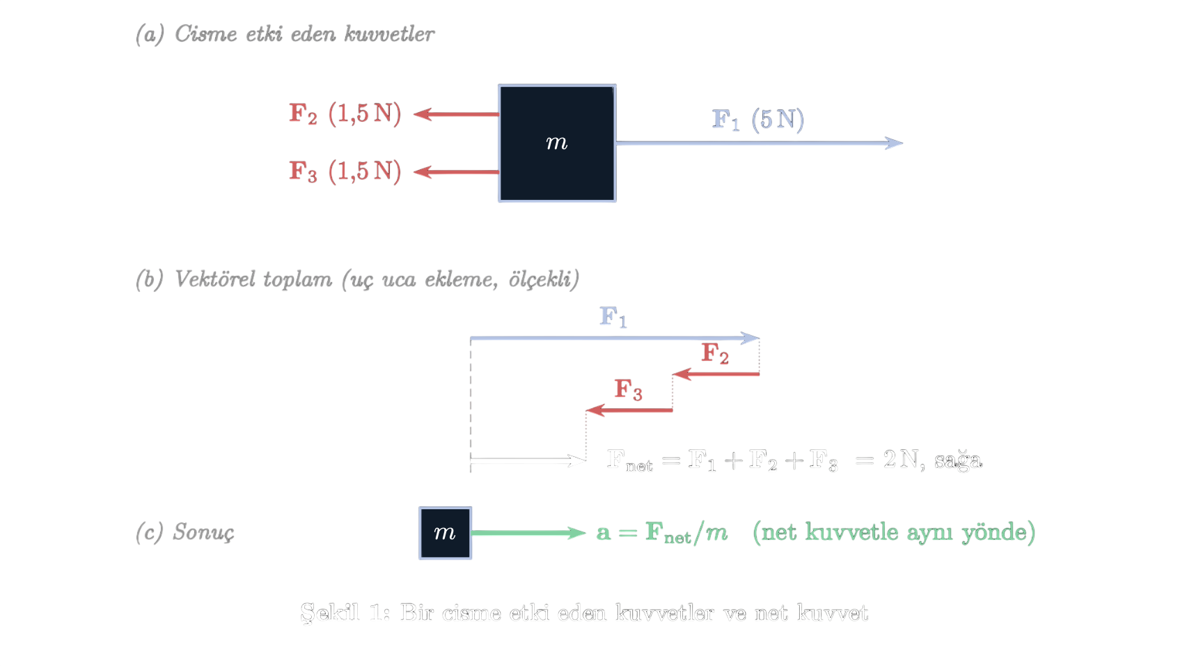
When all the forces are added vectorially, if the rightward force is larger, the object accelerates to the right. The direction of acceleration is always the same as the direction of the net force.

Third Law: Action and Reaction

If two bodies exert forces on one another, those forces are equal in magnitude and opposite in direction.

For example, if the force exerted by body 1 on body 2 is $\mathbf{F}_{12}$, then:

$$\mathbf{F}_{12} = -\mathbf{F}_{21}$$

If an object is pushed to the right, the object pushes back on the source of the push with an equal force to the left. Read together with the second law, the third law has an important consequence: the momentum changes of the two bodies cancel one another at every instant, so the total momentum of a system is conserved when no external force acts on it.

Law of Gravitation

Using these three laws, Newton’s law of gravitation can be written down. For two bodies of masses $m_1$ and $m_2$ separated by a distance $r$, the magnitude of the gravitational force is:

$$F = G\,\frac{m_1 m_2}{r^2}$$

Here $G$ is the universal gravitational constant:

$$G = 6.674 \times 10^{-11}\ \text{N}\cdot\text{m}^2/\text{kg}^2$$

A three-body system can be imagined as follows: two stars orbit one another to form a binary-star system, while a planet orbits around that system. Between every pair of bodies there is an action–reaction force pair obeying the law above. The motion of each body is determined by the net force acting on it.

Instantaneous Action at a Distance (Nonlocal Structure)

An important feature is hidden in the form of the gravitational law.

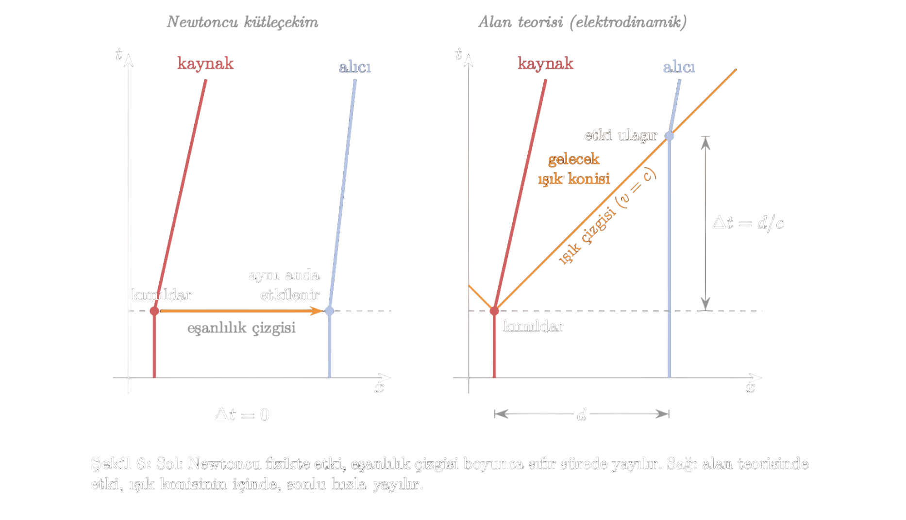
In Newton’s law of gravitation, the force depends on the instantaneous positions of distant particles; there is no time delay or propagation speed.

This is easy to see in the formula: nowhere in $F = G\,m_1 m_2 / r^2$ does time appear. The formula says: wherever $m_2$ is now, the force acting on $m_1$ is determined by that position now. For example, if the Sun were suddenly displaced slightly, Newton’s law would say that the change in Earth’s orbit would begin not after the roughly eight minutes required for light to travel from the Sun to Earth, but at that very instant; the influence would cross the roughly 150 million kilometers of empty space in zero time:

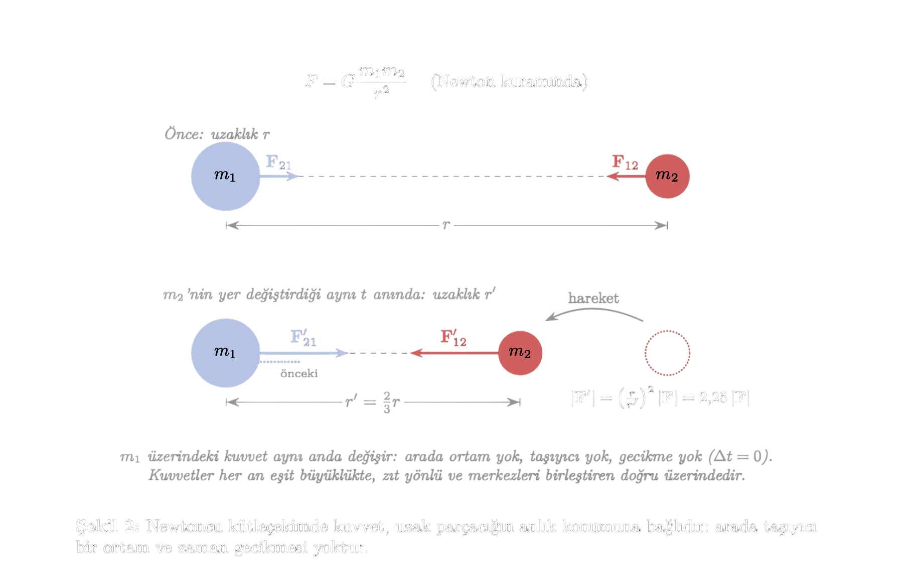
Today, this feature is called nonlocality. Its opposite, locality, is a principle much closer to ordinary intuition: no influence jumps instantaneously across empty space; an influence can propagate only from neighbor to neighbor, step by step, at a finite speed. This principle will be developed in detail in later articles in the series.

Newton’s Philosophical Objection

This feature troubled the creator of the theory himself.

Newton himself regarded instantaneous action at a distance through empty space, without any mediating medium between bodies, as physically unacceptable and viewed his theory of gravitation as a provisional rather than final model.

This is one of the most striking historical details in physics: one of the clearest objections to instantaneous action at a distance came from the very person whose theory contained it. In his letters to Richard Bentley, Newton explicitly described the idea that one body could act on another distant body without anything in between as an “absurdity.” His own position was cautious: he did not propose a mechanism for how gravity was transmitted — in his famous phrase, “I frame no hypotheses” (hypotheses non fingo) — but he acknowledged that the law worked perfectly in calculation. In other words, Newton was confident that his theory made correct predictions, but he believed that the physical reality behind those predictions was not yet known. For him, the law of gravitation was not a final explanation; it was a provisional model valid until the true explanation — a mediator carrying the influence — could be found.

Newtonian Space and Time

The Newtonian worldview has a dimension even deeper than its laws: what it says about space and time themselves. To illustrate this, we can draw a spacetime diagram. The vertical axis represents time, while the horizontal axis represents space. The worldlines of the binary-star and planet system mentioned above can also be added to the diagram:

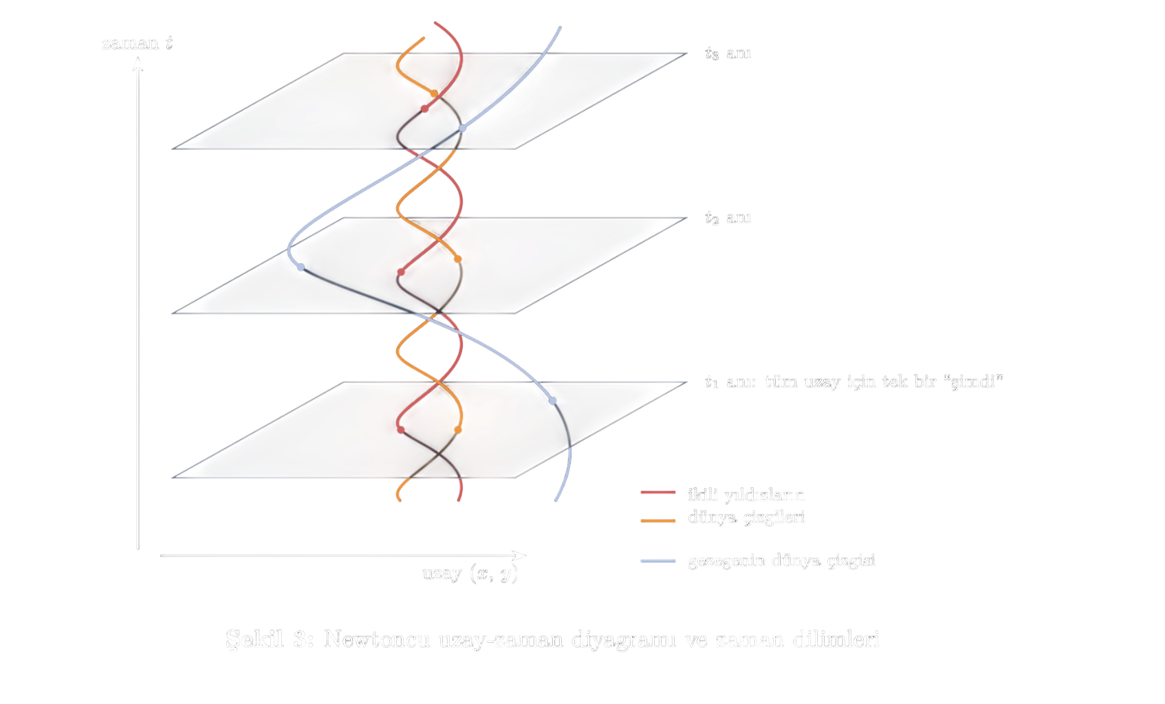
In Newtonian physics, at any instant $t$, there is a definite time slice cutting straight across all of space:

For every instant $t$, there is a single “now” slice that spans the entire universe.

Time flows upward, and every instant is defined simultaneously throughout all of space. Einstein’s relativistic corrections do not appear in this picture; the phrase “right now” has the same meaning at every point in the universe.

A historical subtlety should be noted here. The statement “gravity is instantaneous” is not a claim about Newton’s personal belief, but an observation about the structure of the law: there is no delay term in the formula, so the theory treats action at a distance as instantaneous. Newton himself, however, as discussed in Section [[#Newton's Philosophical Objection|4.8]], regarded this feature as physically unacceptable and left open the question of how the influence was transmitted. Thus, when we say “Newtonian gravity is nonlocal,” we are describing the structure of the theory, not the metaphysical preferences of its founder.

There is a second subtlety. The absolute simultaneity ,shown in Figure 3, disappears in special relativity. There, whether two events are simultaneous depends on the observer; there is no single “now” slice cutting across the entire universe. Those slices are therefore a feature of the Newtonian picture, not the final word of classical physics.

In this series, when we refer to the “classical view,” Einstein’s special relativity will generally be included as well. In other words, we assume that there is a maximum speed in the universe that nothing can exceed:

$$v \leq c, \qquad c = 3 \times 10^{8}\ \text{m/s}$$

Why this matters will become clear later: the conflict between quantum mechanics and classical intuitions about locality and causality appears precisely here — where entanglement confronts the speed-of-light limit. In famous quantum thought experiments such as the Einstein–Podolsky–Rosen (EPR) paradox, for example, two quantum particles are entangled and then separated by a large distance, and a measurement performed on one appears to produce an instantaneous effect on the other. Situations of this kind put the classical principle of locality into question and raise the issue: “In the quantum era, is nature really local?” These striking examples will be examined in detail in later parts of the series.

Maxwellian Electrodynamics

The second pillar of the classical worldview is electrodynamics. As with gravitation, we begin with a force law.

Coulomb’s Law

For two point charges $q_1$ and $q_2$ separated by a distance $r$, the electrostatic force is:

$$F = k\,\frac{q_1 q_2}{r^2}, \qquad k = \frac{1}{4\pi\varepsilon_0} = 8.99 \times 10^{9}\ \text{N}\cdot\text{m}^2/\text{C}^2$$

Notice that this expression has exactly the same mathematical structure as Newton’s law of gravitation: both are inverse-square laws. Masses are replaced by charges, and $G$ is replaced by $k$. The only important difference is that electric charge can have either sign: opposite charges attract, while like charges repel. Gravity, by contrast, is only attractive.

Electric Field and Superposition

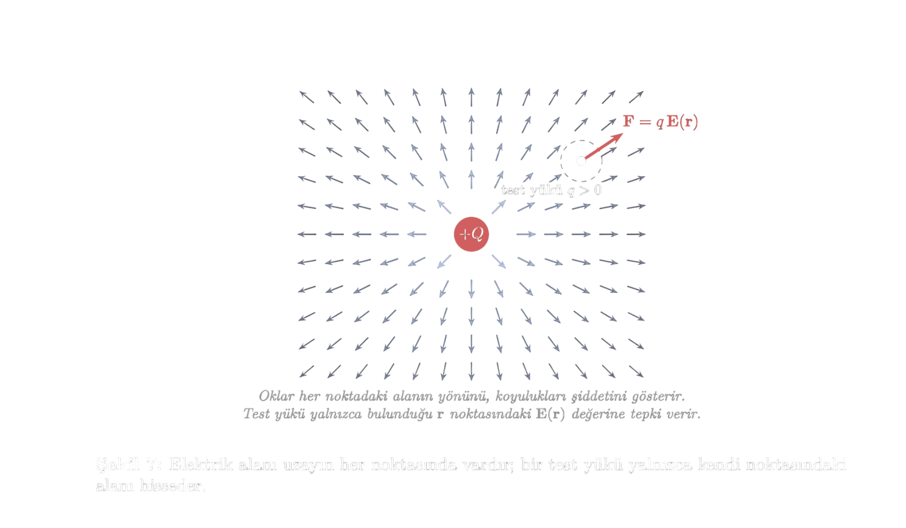
If the Coulomb force is divided by one of the charges, we obtain the concept of the electric field:

$$\mathbf{E} = \frac{\mathbf{F}}{q}$$

The physical meaning of the electric field is this: “If a test charge were placed at that point, how much force would it feel per unit charge?” By placing an imaginary small test charge at a point in space and examining the force acting on it, we can measure both the magnitude and the direction of the field.

If there are several source charges, the total electric field at a point is the vector sum of the contribution from each charge. This is called the principle of superposition:

$$\mathbf{E}(\mathbf{r}) = \sum_{i} \frac{1}{4\pi\varepsilon_0}\,\frac{q_i}{|\mathbf{r} - \mathbf{r}_i|^2}\,\hat{\mathbf{r}}_i$$

Here $\mathbf r$ denotes the point where the field is calculated, $\mathbf r_i$ denotes the position of the $i$th source charge, and $\hat{\mathbf r}_i$ is the unit vector pointing from that charge toward the point at which the field is being evaluated.

Consider an example. Suppose a weak source charge $q_1$ and a stronger source charge $q_2$ act on a test charge in opposite directions:

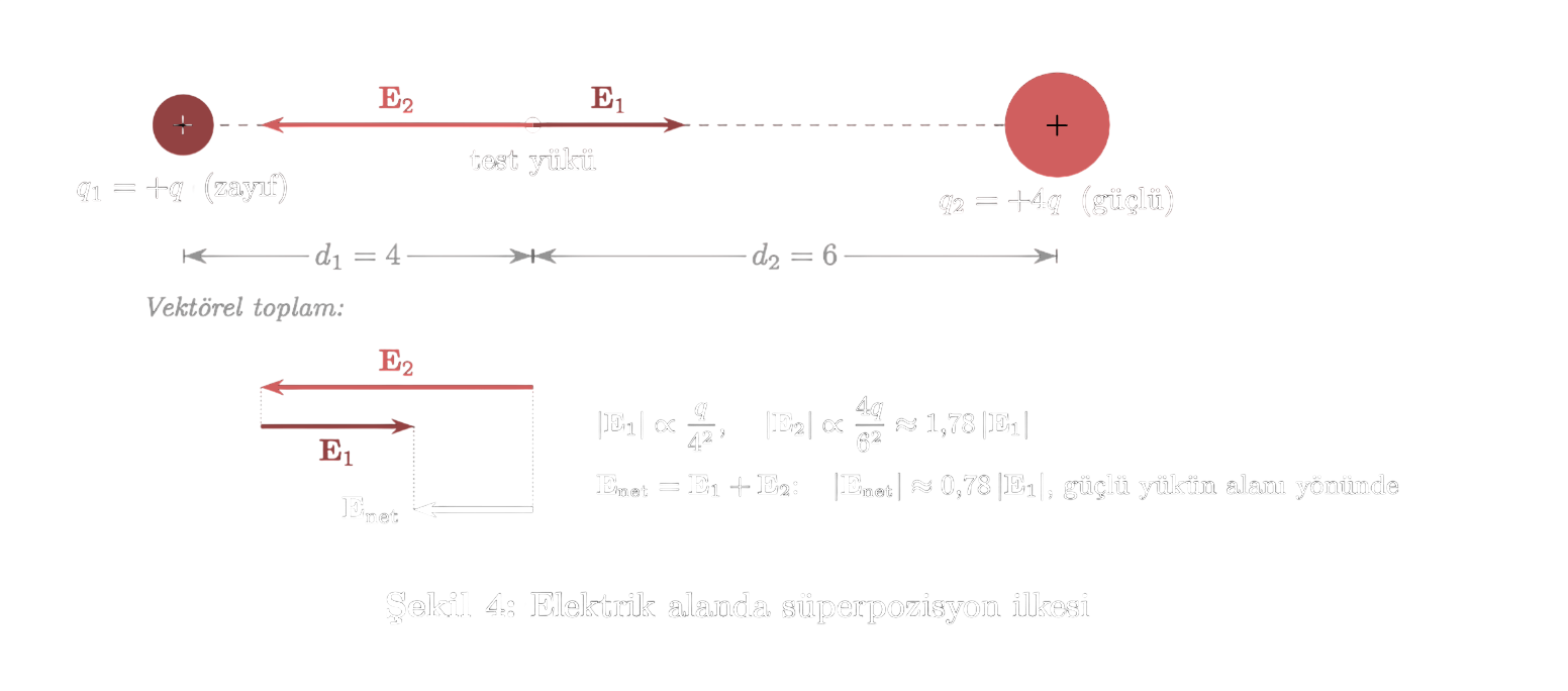
The two fields partially cancel, and the net field remains in the direction of the stronger one. This is exactly what the superposition principle says.

Maxwell’s Equations

We can now move to the heart of electrodynamics. Maxwell’s equations may look intimidating at first, but what they say is actually quite simple. There are four equations, and they can be divided into two groups: the first two describe how fields arise from charges and what forms those fields can take, while the last two describe how fields are generated by currents and by changes in one another.

To read the equations, we first need to define two mathematical operations:

Definition (Divergence). The divergence $\nabla \cdot$ of a vector field at a point measures the net amount by which the field spreads outward from that point. If more field lines enter a region than leave it, the divergence is negative; if fewer enter than leave, it is positive.

Definition (Curl). The curl $\nabla \times$ of a vector field at a point measures the tendency of the field to form closed loops around that point.

We can now write the four equations one by one.

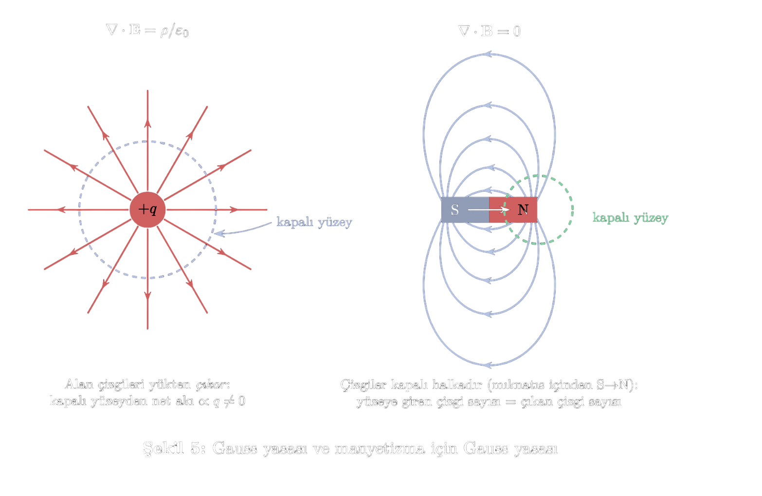
Gauss’s Law

$$\nabla \cdot \mathbf{E} = \frac{\rho}{\varepsilon_0}$$

This equation says that the electric field spreads outward from charge density. Here $\rho$ is the charge density — the amount of charge per unit volume in a region. The more charge a region contains, the stronger the field spreading outward from that region; the sign of the charges determines the direction of that spreading. At a point containing a single small charge, the divergence is small; at a point where many charges are concentrated in the same region, it is larger.

Gauss’s Law for Magnetism

$$\nabla \cdot \mathbf{B} = 0$$

This equation says that such outward spreading is not possible for the magnetic field. Magnetic field lines always form closed loops: the field lines around a magnet pass through the magnet and close back on themselves. As a result, the number of magnetic field lines entering any region of space is always equal to the number leaving it — the divergence is zero. (In other words: there are no magnetic monopoles.)

These two equations can be summarized side by side in a diagram:

Ampère’s Law

$$\nabla \times \mathbf{B} = \mu_0 \mathbf{J} + \mu_0 \varepsilon_0 \frac{\partial \mathbf{E}}{\partial t}$$

This equation says that the magnetic field — which always forms closed loops, which is why we take its curl — is generated by two sources:

1. Moving charges: $\mathbf{J}$ is the current density. Charges moving through a wire generate a loop-shaped magnetic field around the wire.

2. A time-varying electric field: If the strength of the electric field in a region increases or decreases with time, that change also induces a magnetic field. The term $\partial \mathbf{E}/\partial t$ expresses exactly this.

Maxwell added this second term to the equation, which is why the law is often called the Ampère–Maxwell law.

Faraday’s Law

$$\nabla \times \mathbf{E} = -\frac{\partial \mathbf{B}}{\partial t}$$

The final equation is almost the mirror image of Ampère’s law: a changing magnetic field induces an electric field in the form of a closed loop.

A common example from introductory physics courses is a wire loop with a magnet moved back and forth through it. As the magnet approaches the loop, the magnetic field at the location of the loop becomes stronger; as it moves away, the field becomes weaker. This change creates an electric field circulating around the loop, and that field drives a real current through the wire. This is exactly the operating principle of generators.

The final two equations can be combined in a single diagram:

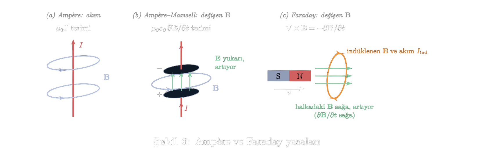
Notice that a “moving” magnetic field and a “changing” magnetic field are really the same thing: when a magnet is moved, an observer at a fixed point in space sees the magnetic field at that point change with time.

The Lorentz Force Law

In addition to Maxwell’s four equations, there is one more law that might be called an “honorary Maxwell equation.” Maxwell’s equations tell us how fields are generated; the Lorentz force law tells us how charged particles respond to those fields:

$$\mathbf{F} = q\mathbf{E} + q\,\mathbf{v} \times \mathbf{B}$$

The first term is the force exerted by the electric field on the charge; the second is the force exerted on a charge moving with velocity $\mathbf{v}$ through a magnetic field. Because of the cross product, the magnetic force is always perpendicular to the velocity — which is why a magnetic field does no work on the charge, but only changes its direction of motion.

The Ontology of Electrodynamics

The universe consists both of particles and of physically real fields ($\mathbf E$ and $\mathbf B$) that fill space and carry energy and momentum in their own right.

This is an important departure from the Newtonian picture of the classical worldview. In the Newtonian inventory there were only particles and forces; electrodynamics adds a new kind of entity to the inventory: fields. Moreover, a field is not merely a mathematical device that makes calculations easier. Maxwell’s equations say that fields can carry energy and momentum on their own and can propagate as waves — at the speed of light; those waves are light itself. A charge does not directly “feel” another distant charge; it feels only the field at its own location and receives the force from that field:

The consequence is important: when a charge moves, a distant charge does not learn about it instantaneously. It learns only when the information has propagated through the field at the speed of light and reaches it. In this way, the instantaneous action that Newton found philosophically unacceptable disappears from electrodynamics; the influence is now local — it propagates from neighbor to neighbor at a finite speed. In a spacetime diagram, the region that can be reached by an influence originating from an event is called the light cone: the edges of the cone trace the paths followed by light, while its interior contains everything that moves more slowly than light. When the two classical conceptions of influence are placed side by side, the difference becomes clear:

The inventory of the classical worldview therefore contains two kinds of entities: particles and fields. One of the first questions to be asked when we move to quantum mechanics will be this: what belongs in the inventory of quantum theory — and where does the wave function fit into that list?

Summary of the Classical View

In this article, we have built up piece by piece what is meant by the “classical-physics worldview”:

$$\text{Classical view} = \underbrace{\text{Newtonian mechanics}}_{\text{3 laws + gravitation}} + \underbrace{\text{Maxwellian electrodynamics}}_{\text{4 equations + Lorentz force}} + \underbrace{\text{special relativity}}_{v \leq c}$$

The ontological inventory is also clear: the classical world consists of particles and of fields that locally mediate the interactions between them.

This framework has three characteristic features:

1. Determinism: If the present state of a system and the forces acting on it are known, the laws determine the future exactly.

2. Realism: Fields and particles are things that exist in the world whether or not anyone is looking at them.

3. Locality: Once special relativity is taken into account, no influence propagates faster than the speed of light. Newton’s law of gravitation is the one exception to this principle; the transformation of gravity into a local field theory is completed only with general relativity.

Quantum mechanics calls each of these three features into question — and in some approaches, all of them at once. The measurement problem puts determinism under pressure: in standard quantum mechanics, measurement outcomes are given only probabilistically. Whether determinism must actually be abandoned, however, depends on the candidate theory; pilot-wave theory remains deterministic, while objective-collapse theories write randomness directly into the fundamental law. The debate over ontology challenges realism at its foundations: is the wave function something that really exists, or is it merely information or probability? Entanglement, meanwhile, creates a deep fracture in the concept of locality: Bell’s theorem and the experiments that followed it show that the correlations between widely separated particles cannot be explained by any local theory. For this reason, the next articles in the series will first develop these issues — locality/causality and ontology/measurement — in detail on the background of classical physics, and then show how those classical foundations are challenged in quantum mechanics.