Feynman Diagrams Part 1

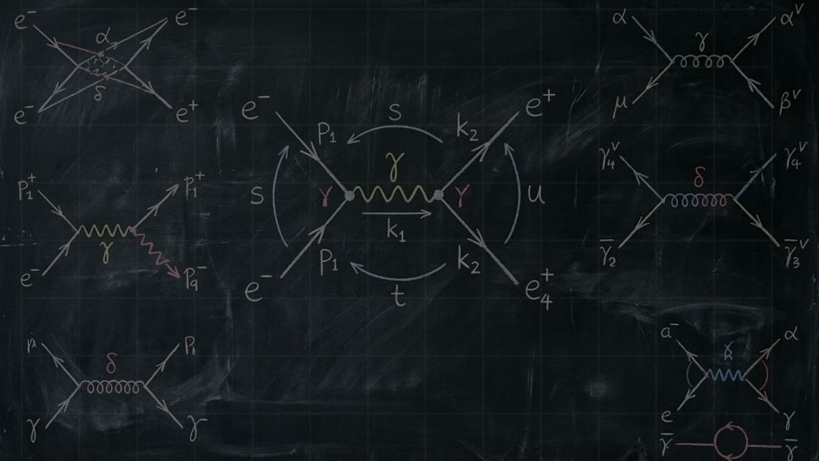
A cosmic message to physicists and a product of Feynman's incisive mind, Feynman diagrams explain particle interactions to us almost perfectly. I say "almost perfectly" because, in some particle interactions, processes that appear to be allowed by Feynman diagrams never occur. We will examine an example of such a model shortly. Let us begin by explaining the most fundamental particle interactions.

Quantum Electrodynamics (QED)

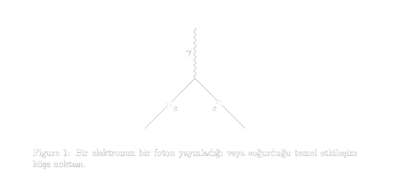
Quantum electrodynamics, Feynman's legacy to us physicists, is, in the simplest terms, a subject in quantum physics that explains electromagnetic phenomena: the interactions between the electrically charged electron and positron through photons, the carriers of the electromagnetic force (also called gauge bosons). Every electromagnetic phenomenon can be reduced to the most fundamental diagram shown below.

In the interaction in Figure 1, time flows from left to right, and what you should see is this: an electron travelling forward in time arrives, interacts with a photon (emits or absorbs a photon), and continues on its way as an electron. This diagram is the most fundamental type of interaction and can be explained as follows: photons are the carrier particles of the electromagnetic field (gauge bosons), and when an electron enters an electric or magnetic field—or both at the same time—it is in fact interacting with photons. As in this example, diagrams reduce far more complex processes to a form simple enough for anyone to understand.

Møller Scattering

The type of interaction known in broadly accessible physics as Coulomb repulsion or the electric force is called Møller scattering in quantum electrodynamics.

Møller scattering is no different from the repulsion between two electrons that we learned about in high school. The Feynman diagram representing this process is as follows:

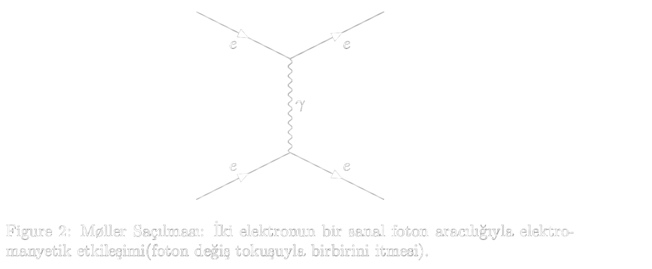
In the interaction in Figure 2, time again flows from left to right (as we will assume throughout this article). In this diagram, two electrons enter, a photon passes from one to the other, and two electrons emerge. As you may have noticed from the label beneath the figure, we call the mediating photon a virtual photon. This is because the mediating photon that transfers momentum and energy between the two electrons cannot be observed directly by our detectors. Calculations and experimental data tell us that this mediator is a photon, but because we cannot observe it, we call it "virtual." It is as if something were there, although there is nothing to be seen!

Bhabha Scattering

What does a "particle travelling forward in time" even mean? The use of that expression suggests that there must also be particles travelling backward in time! Let us explain this using our elegant inheritance, Feynman diagrams:

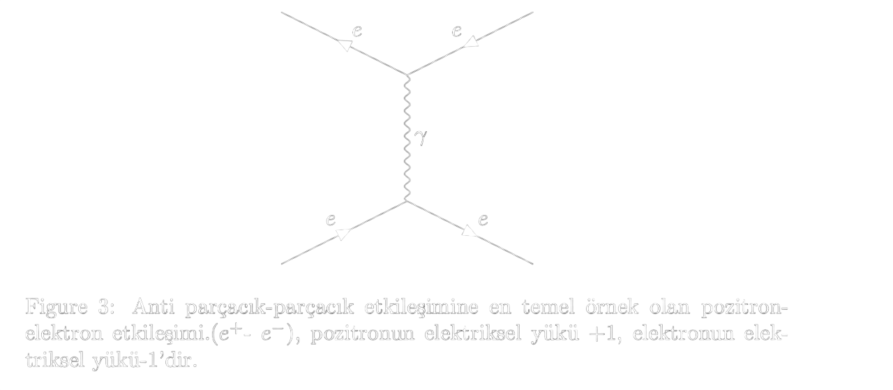
In Figure 3, where time flows from left to right, you see a particle moving in the opposite direction along the time axis. This particle is the positron, the antiparticle of the electron. In Feynman diagrams, particles travelling backward in time are treated as antiparticles, as in the positron example. In this interaction, a photon is exchanged between a positron and an electron; they attract each other through the electric force and collide, then annihilate each other to create a photon, which subsequently produces a new electron–positron pair. (The newly formed positron–electron pair arises through energy–mass conversion in accordance with Einstein's $E=\gamma mc²$ and the energy–momentum relation $E=pc$ for massless particles.) The positron is not very different from the electron. They both have the same mass, which, expressed in kilograms—the unit we use in the macroscopic world—is

$$m_e \approx 9,109 \times 10^{-31} kg$$

In particle physics, and expressed in terms of energy on the basis of Einstein's $E=\gamma mc²$ formula, it is correct to write

$$m_e \approx 0,511 MeV/c^2$$

Both quantities correspond to mass and are exactly the same for the electron–positron pair. Not only their masses but also their spins are the same, and both are fermions with spin 1/2. Both are stable particles in isolation; they do not decay spontaneously into other particles. They are not composed of combinations of quarks, as protons and neutrons are. Like quarks, the electron and positron are "made of their own pure substance." In other words, each consists of itself. One point must be emphasized here: electric charge is not the sole basis of the matter–antimatter duality. Neutrinos, for example, do not carry electric charge, yet antineutrinos exist. The muon neutrino and muon antineutrino, the electron neutrino and electron antineutrino, and the tau neutrino and tau antineutrino are examples. The fundamental reason a particle is "anti" is that all the charge-like quantum numbers defining that particle have the opposite sign. As you can see in our diagram in Figure 3, the particle travelling backward in time is the antiparticle, and this is how we describe the matter–antimatter duality. Of course, diagrams allow us to model many different particle interactions. The following diagrams are further examples:

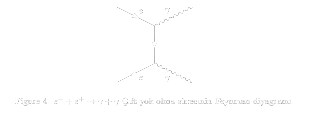
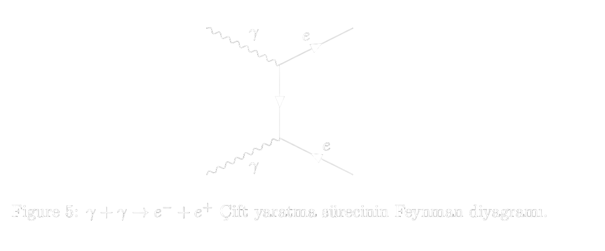
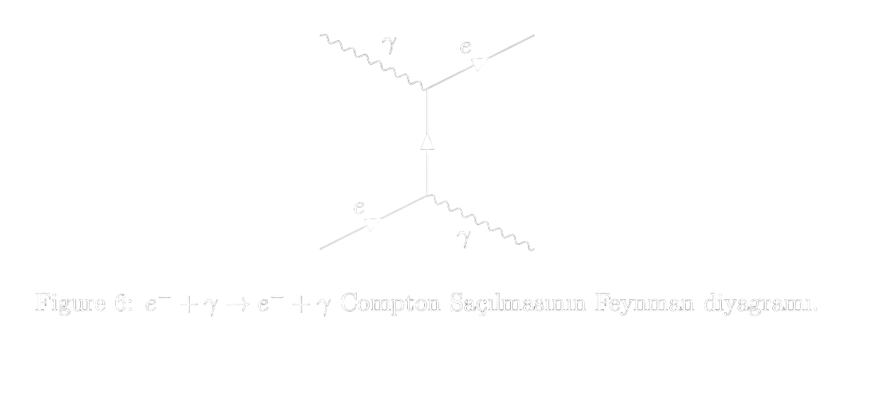
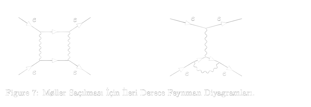
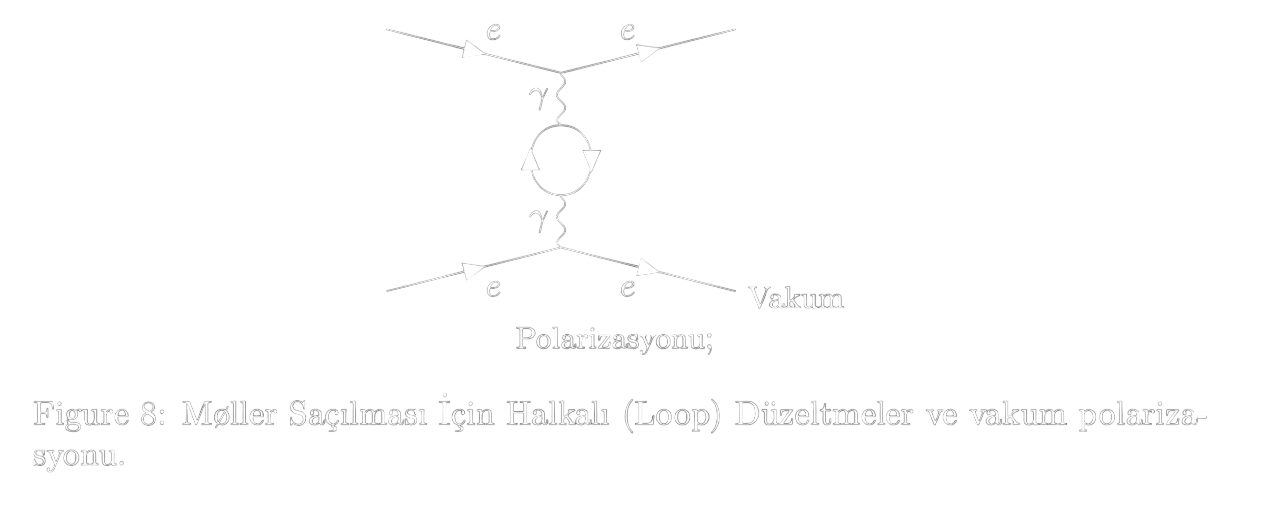
In each of these diagrams, two electrons enter the process and two electrons emerge. Reactions of this kind are called Møller scattering and represent the repulsion of like charges. The internal lines in a diagram represent particles that come into and out of existence momentarily during the process without changing the interaction. These are virtual particles and are not observed. Only the external lines represent "real," observable particles. The external lines tell us which physical process occurs, while the internal lines describe the mechanism underlying that process.

Feynman diagrams are only a model, and although the horizontal axis in diagram space represents time, the vertical axis does not represent the distance between particles. The Feynman rules state that energy and momentum must be conserved at every point in the diagram. Under these rules, the "primitive vertex" in which an electron interacts with a photon—the "most fundamental diagram" shown first in this article—cannot model a possible physical process. As I noted at the very beginning of the article, some particle interactions that appear modelable with Feynman diagrams do not occur in nature. We can draw the diagrams, but the mathematical calculations hidden behind them give a result of "zero." The reason is entirely kinematic. For example, the reaction $e⁻ \to e⁻ + \gamma$ violates energy conservation. In the center-of-mass frame, the electron is initially at rest, so its energy is the "rest-mass energy" $mc²$. In this state, the electron cannot decay into a photon and a recoiling electron, because the recoiling electron alone would require an energy greater than $mc²$ (as required by the conservation of energy and momentum).

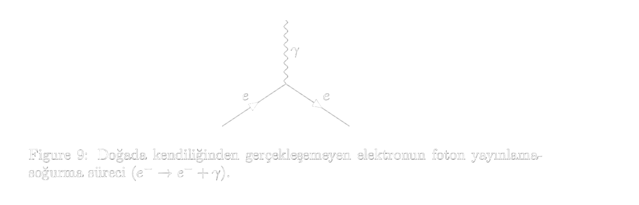
Although these reactions cannot occur, they are extremely helpful for grasping the subject in the simplest possible way at the beginning of one's education. As you will have noticed, I began my own article by explaining them, which is why I felt the need to say "almost perfectly." Returning to our subject, another reaction that appears possible in the diagrams but is not possible in high-energy physics is $e⁻ + e⁺ \longrightarrow \gamma$:

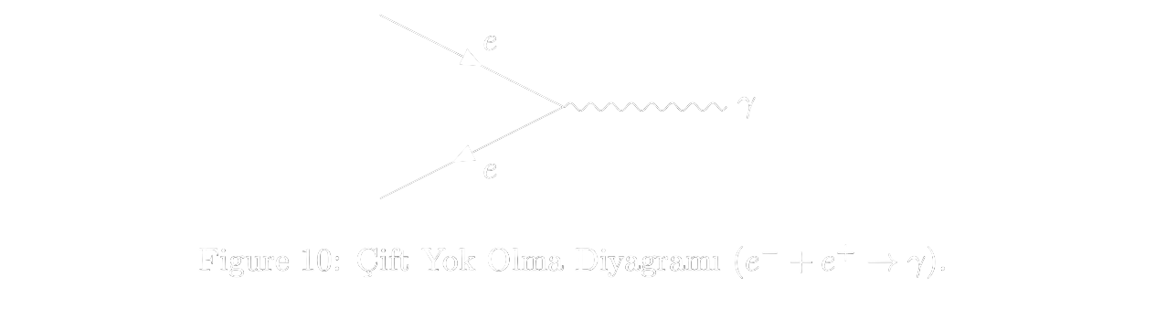
This reaction is not kinematically possible. In the center-of-mass frame, the electron and positron approach with equal speeds in opposite directions, so the momentum before the collision is zero. Photons, however, always travel at the speed of light in vacuum, and therefore the final momentum cannot be zero. An electron and a positron can undergo pair annihilation and produce two photons, but they cannot produce a single photon.

In Closing...

In this article, I aimed to present Feynman diagrams to readers without mathematical expressions. Of course, diagrams encompass far more than this. In this introductory article, I wanted to convey the importance of the role played by Feynman diagrams in quantum electrodynamics. Our next subject will be the quantum field known as quantum color dynamics, or quantum chromodynamics (QCD), where there will naturally be plenty of further examples of Feynman's legacy: Feynman diagrams. A few articles from now, we will also begin working through the mathematical operations hidden in the background, known as Feynman calculus or the Feynman calculation technique. I wish you success and enjoyable reading.

References

1. David Griffiths, Introduction to Elementary Particles (Second, Revised Edition)
2. The teachings and lecture notes of Prof. Dr. Muhammed Deniz