Electromagnetic Theory Part 2

Electromagnetic Theory — Part 2

1. Introduction

Hello, everyone. Today we will solve examples in order to gain a better grasp of the laws we learned in the first part. We will examine methods for calculating the electric field and potential, as well as the Laplace and Poisson equations whose solutions we postponed discussing in the first part.

2. Electric Field and Potential

First, let us recall the relation between the electric field and potential that we gave in the first part:

$$\vec{E} = -\nabla V = -\left\langle \frac{\partial V}{\partial x},\, \frac{\partial V}{\partial y},\, \frac{\partial V}{\partial z} \right\rangle$$ $$V(\vec{r}) = -\int_{\mathcal{O}}^{r} \vec{E} \cdot d\vec{l}$$

When the potential function is given, we can take its gradient and multiply by minus one to obtain the electric-field vector. Likewise, we can calculate the potential of a point separated from the origin by the position vector $r$ using the equality given by the line integral of the electric field.

To calculate the electric field, we use Gauss's law, namely

$$\nabla \cdot \vec{E} = \frac{\rho}{\epsilon_0} \qquad \oint_{\partial V} \vec{E} \cdot d\vec{S} = \frac{\sum Q}{\epsilon_0}$$

In electrostatics problems, we generally try to determine the electric field from a charge distribution. When there is symmetry, and the electric field is constant over certain chosen surfaces so that it can be taken outside the integral, Gauss's law allows us to find the electric field easily.

Why potential?
What if there is no symmetry? What if we cannot simply take the field outside the integral? Since the field is a vector, dealing with calculations of its components will also be complicated. It is much easier to calculate a scalar, such as the potential, and then pass to the electric field.

Let us begin this part by examining the Laplace and Poisson equations with which we concluded the first part.

3. Laplace's Equation

$$\boxed{\nabla^2 V = \frac{\partial^2 V}{\partial x^2} + \frac{\partial^2 V}{\partial y^2} + \frac{\partial^2 V}{\partial z^2} = 0}$$

We have a partial differential equation. Let us first examine it in one dimension.

$$\frac{d^2 V}{dx^2} = 0$$

We now have an ordinary differential equation in one variable. The second derivative of the potential function is zero. Recalling our knowledge of calculus, a zero derivative means that our expression is constant. Thus, the first derivative must be a constant number. Let it be, for example, the real number $a$. If the derivative of the potential is $a$, we can integrate our expression and obtain

$$V(x) = ax + b$$

All potential expressions in the form of a linear function, with $a$ and $b$ real numbers, satisfy Laplace's equation. The electric field, forces, and so forth can of course be found from this. The electric field is

$$\vec{E} = -\nabla V = -\frac{dV}{dx} = -a$$

The calculation is straightforward in one dimension. We need two arbitrary constants for the solution.

Now let us consider two dimensions.

$$\frac{\partial^2 V}{\partial x^2} + \frac{\partial^2 V}{\partial y^2} = 0$$

We no longer have an ordinary differential equation in one variable, but a partial differential equation. This means that the equation no longer has a general solution. Above, we found the general solution of the second-order differential equation in one dimension using two constants. The multidimensional equation we now have does not possess a general solution, because its solutions are infinitely varied and cannot be placed into a single form.

The geometric meaning of the Laplacian
What did the Laplacian mean? It was proportional to the difference between the value of the function and the average of the values at the surrounding points. Since our equality is zero, there is no difference between the value of our function and the average of its surrounding values. In other words, if I take a circle, the average of the values along the circle equals the value at the center of the disk.

From this, we can infer that no point can be a maximum or minimum. Laplace's equation produces the smoothest surface, with the least variation, that can satisfy the boundary conditions. There are neither peaks (maxima) nor valleys (minima). Just as the shortest distance between two points is a straight line, the solution of Laplace's equation in two dimensions represents the surface of smallest area spanning the given boundary curve. I hope this also makes our finding of a linear equation in one dimension more intuitive.

You might ask why we bother if there is no general solution. The absence of a general solution does not mean that we cannot solve the equation. We will solve partial differential equations using the boundary conditions of the function we seek. We will discuss methods for doing so in this part.

The same reasoning applies in three dimensions. This time, if we draw a spherical shell, we can say that the average value on its surface must equal the value at the center of the sphere. For the same reasons, the solution again has no maximum or minimum. We can now proceed to the methods of solution.

4. Boundary Conditions and the Uniqueness Theorem

Infinitely many solutions can satisfy Laplace's equation. To determine which one belongs to our problem, we must know how the function behaves under certain conditions. For the one-dimensional expression $ax+b$ that we found, for example, if we are given the value of the function at two different points, or its derivative and its value at one point, we can determine the unique solution exactly. Suppose, however, that we are given the derivative at two points. Since the derivative of our function is constant, different values for the two derivatives would be contradictory and there would be no solution. If the same value were given twice, repeating the same information would make no contribution to the solution. These constraining conditions, or boundary conditions, must therefore be chosen carefully.

Boundary condition:
In its simplest form, a boundary condition is information specifying the value taken by the function at the edges—the boundary or surface—of the region in which the solution is sought.

Note: The Uniqueness Theorem and Its Proof:
The uniqueness theorem tells us that there is a unique function satisfying a consistent set of boundary conditions. Let us prove it.

Suppose that we have two functions, $V_1$ and $V_2$, satisfying the boundary condition. Define a new function $V_3 = V_1 - V_2$. Since they satisfy Laplace's equation,

$$\nabla^2 V_1 = 0 \qquad \nabla^2 V_2 = 0$$

Differentiation is linear and distributes over addition. Therefore,

$$\nabla^2 V_3 = \nabla^2 V_1 - \nabla^2 V_2 = 0$$

Now consider the boundary conditions. By our initial assumption, $V_1$ and $V_2$ are equal on the boundary. This means that $V_3$ is $0$ on the boundary. Since the function has no minimum or maximum, it cannot take the value zero, then other values, and then zero again; to do so, it would need a point at which it increased and then decreased—that is, a maximum or minimum. Our function must therefore be zero everywhere:

$$V_3 = V_1 - V_2 = 0 \;\longrightarrow\; V_1 = V_2$$

Thus, the function satisfying the boundary conditions is indeed unique.

Also valid for Poisson's equation
Before proceeding, let us note that this also holds for a solution of Poisson's equation:

$$\begin{aligned} \nabla^2 V_1 &= -\frac{\rho}{\epsilon_0} \\ \nabla^2 V_2 &= -\frac{\rho}{\epsilon_0} \\ \nabla^2 V_3 &= \nabla^2 V_1 - \nabla^2 V_2 = -\frac{\rho}{\epsilon_0} + \frac{\rho}{\epsilon_0} = 0 \end{aligned}$$

What we learn from this theorem is that if we have found a potential satisfying the boundary conditions and Laplace's equation (or Poisson's equation), it is the solution we seek.

5. Method of Images

In this method, we will use the result we have just obtained. Suppose that we have a charge distribution whose calculation is difficult, and we want to determine its potential. Let us proceed through an example. Imagine an infinite grounded conducting surface. Let a charge $+q$ be located above this surface at the point $(0,0,d)$:

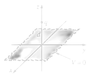
It seems very easy—is it not simply $kq/r$? It is not. The surface is conducting. Even though the net charge of the surface is zero, our charge $+q$ attracts the negative charges on the surface and repels the positive ones, producing an induced charge distribution over the surface. In other words, there is a charge distribution that cannot be found easily, and we are looking for the potential. Wonderful.

Our first task here is to determine the boundary conditions.

What does grounded mean?
We take the ground to be zero. If a point on the surface has a potential difference relative to the ground—that is, relative to zero—an electric field immediately arises, and charge flows until the difference disappears. In short, it means that the potential on our surface is zero.

Our boundary conditions are:

1. If $z=0$, then $V(x,y,z) = 0$ must hold.
2. If we move very, very far from the origin, we also move very far from both the charge $+q$ and the induced charges on the surface, and our potential approaches zero: if $x^2 + y^2 + z^2 \gg d^2$, then $V \to 0$.

The theorem now tells us that if we find a function satisfying these two conditions, it is the potential function we seek. I have a suggestion: let us place a charge $-q$ a distance $d$ below the origin:

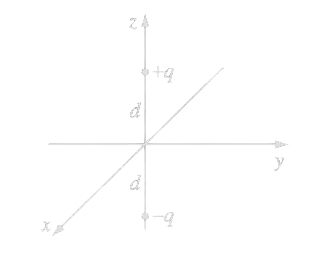
If we do this, symmetry makes the potential zero when $z=0$. Potential is a scalar; for $z=0$, that is, on our surface, every point is equidistant from the charges $+q$ and $-q$. Their contributions cancel, making the potential zero. Moreover, with two charges at a distance $d$ from the origin, the potential decreases and approaches zero as we move very far away. We had two conditions, and both are satisfied.

To express this situation, consider our potential expression:

$$V = \frac{1}{4\pi\epsilon_0} \sum_i^n \frac{q_i}{|\vec{d}_i|}, \qquad \vec{d}_i = \vec{r} - \vec{r}_i$$

Finding the distances:
We must find the distance from each charge to the field point. First consider $+q$. Since it is at zero in the $x$ and $y$ directions, the distance between us and the charge along the $z$-axis is, by the Pythagorean theorem and elementary geometry, $z-d$. By the same reasoning, it is $z+d$ for the charge $-q$, because for a point a distance $d$ below the origin and a point a distance $z$ above it, the total separation is $z+d$. (You might ask what happens if $z$ is negative, if we are below the charge, and so on—the result does not change; the expressions remain the same.) To obtain the length, we add the squares of the separations along the axes.

The result obtained from the potential expression is

$$\boxed{V(x,y,z) = \frac{1}{4\pi\epsilon_0}\left[ \frac{q}{\sqrt{x^2+y^2+(z-d)^2}} - \frac{q}{\sqrt{x^2+y^2+(z+d)^2}} \right]}$$

Since this expression satisfies both conditions, we have found the potential we seek.

Method of images:
The method of images consists of satisfying the boundary conditions using fictitious charges that we introduce in order to find the solution, and then identifying the solution by virtue of the uniqueness theorem.

We found the solution easily without having to deal with that complicated charge distribution. You may still be curious about the distribution, however. Let us show a short method for calculating it.

Induced Charge Density

Electric field inside conductors:
The electric field inside conducting surfaces is zero. If the electric field inside were not zero, charges would move and eventually come to rest on the surface after cancelling the electric field. If the electric field is zero, then, as we can infer from Gauss's law, the net charge density is also zero. Thus, the net amount of charge inside conductors is zero. (The converse, incidentally, is not true: the electric field need not be zero when the net charge is zero.) This is also why your phone loses reception in an elevator.

Consider the surface of the conductor, and suppose that the electric field makes an angle $\theta$ with the surface. It would then have components parallel and perpendicular to the surface. A parallel component would mean that the charges were not stationary on the surface but continued to move. Let us suppose, however, that we have left the charges to themselves and they have reached equilibrium. In this case, there is no longer a component parallel to the surface, precisely because the charges are already in equilibrium. This means that the electric field is perpendicular to the surface.

Returning to Gauss's law, consider the projection of the electric field along the surface normal. Because $d\vec{A}$ already points in the direction normal to the surface, their dot product is simply the product of their magnitudes:

$$\int \vec{E}_n \cdot d\vec{A} = E_n A = \frac{Q}{\epsilon_0} = \frac{\sigma A}{\epsilon_0}$$

Here, the subscript $n$ indicates that the electric field points along the surface normal; we have written the amount of charge as the surface charge density times the area. The areas cancel:

$$\sigma = E_n \epsilon_0$$

Recalling that the electric field is the gradient of the potential,

$$\vec{E} = -\nabla V, \qquad E_n = -\frac{\partial V}{\partial n}$$ $$\boxed{\sigma = -\epsilon_0 \frac{\partial V}{\partial n}}$$

The charge density can be calculated in this way from the potential or electric field. If you calculate it from the potential above and then calculate the total charge from the charge density, the answer is $-q$: the charge $+q$ above the surface has induced a charge of $-q$.

6. Separation of Variables

Another idea we use to solve partial differential equations is separation of variables. We cannot apply it in one dimension because there are no distinct variables to separate. Let us first understand the idea of separation of variables for ordinary differential equations; when we then move to two dimensions, you will already find yourself in a mathematics lesson.

Separation of variables in ODEs:
Suppose that we have variables $x$ and $y$. We examine whether the derivative can be written in separable form. Let $X = X(x)$ be a function of $x$ and $Y = Y(y)$ a function of $y$:

$$\frac{dy}{dx} = X(x)\,Y(y)$$

Moving the function $Y$ below $dy$ and $dx$ to the other side gives

$$\frac{dy}{Y(y)} = X(x)\,dx$$

We now integrate both sides and solve. This is a method for solving an ordinary differential equation.

Let us now turn to the real matter. We will try the same method in two dimensions. Remember that our aim is to solve Laplace's equation:

$$\frac{\partial^2 V}{\partial x^2} + \frac{\partial^2 V}{\partial y^2} = 0$$

Suppose that we write $V$ as a product of functions of the variables $x$ and $y$. This is actually a restrictive case. The expression $3x - 7y^2$, for example, cannot be separated into factors depending on $x$ and $y$. Many expressions we encounter cannot be separated. You may ask, "How will we know whether it can be separated?" You will not. We will assume that it can, try it, and if we reach a final expression satisfying the conditions—congratulations, our assumption was correct.

The separation procedure:

$$V = X(x)\,Y(y)$$ $$Y\frac{d^2X}{dx^2} + X\frac{d^2Y}{dy^2} = 0$$ $$\frac{1}{X}\frac{d^2X}{dx^2} + \frac{1}{Y}\frac{d^2Y}{dy^2} = 0$$

Now things become interesting. Our variables $x$ and $y$ are independent of each other—that is precisely why we use them as coordinates. If $x=7$, for example, $y$ can be anything because it does not depend on $x$. In the equation we have obtained, one term depends only on $x$ and the other only on $y$, yet their sum is zero. Each must therefore be a constant in its own right. If the terms were not constant, a change in one would require the other to change in order for their sum to remain zero. Since they are independent, the only possibility is that both are constant:

$$\frac{1}{X}\frac{d^2X}{dx^2} = C, \qquad \frac{1}{Y}\frac{d^2Y}{dy^2} = -C$$ $$\frac{d^2X}{dx^2} = CX, \qquad \frac{d^2Y}{dy^2} = -CY$$

We now have two ordinary differential equations. Clearly, depending on the sign of $C$, one will receive a minus sign and the other a plus sign. If you have a foundation in differential equations, you know that the solution of a system in which a function's second derivative is a multiple of the function itself is either trigonometric or exponential. In this case, the substitution $C = k^2$ is useful:

$$\frac{d^2X}{dx^2} = k^2 X, \qquad \frac{d^2Y}{dy^2} = -k^2 Y$$

The solutions are

$$\begin{aligned} X(x) &= Ae^{kx} + Be^{-kx} \\ Y(y) &= C\sin(ky) + D\cos(ky) \end{aligned}$$ $$\boxed{V(x,y) = \left(Ae^{kx} + Be^{-kx}\right)\left(C\sin(ky) + D\cos(ky)\right)}$$

What follows depends on the boundary conditions. If the potential decreases with distance, for example, then $A=0$ must hold. If we know the value it takes for a particular $x,y$, its symmetries, and so forth, the boundary conditions allow us to determine the numbers $A, B, C, D,$ and $k$. The system does not change in three dimensions. This time, we bring it into a form such as

$$\frac{d^2X}{dx^2} = (k+l)^2 X, \qquad \frac{d^2Y}{dy^2} = -k^2 Y, \qquad \frac{d^2Z}{dz^2} = -l^2 Z$$

and solve using the boundary conditions.

Example: The Griffiths Problem

Example: Potential between grounded plates
I actually found many excellent examples online, but I think the example in Griffiths's book is especially good, both because of the length of the mathematics and because it looks difficult at first sight. We will solve that one.

In this problem, there are two infinitely long grounded plates at $y=0$ and $y=a$. At $x=0$, there is also an insulating plate joining the two plates, whose potential depends on $y$ and is given by $V_0(y)$.

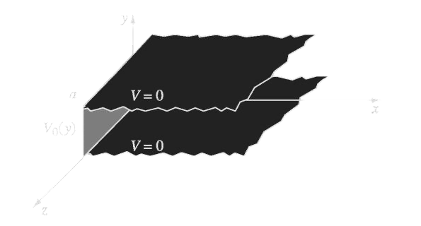
Let us proceed from the general solution that we found above:

$$V(x,y) = \left(Ae^{kx} + Be^{-kx}\right)\left(C\sin(ky) + D\cos(ky)\right)$$

Let us list our boundary conditions:

• If $y=0$, then $V=0$
• If $y=a$, then $V=0$
• If $x=0$, then $V=V_0(y)$
• As $x$ increases, $V$ decreases, and when $x \to \infty$, $V=0$

The first two conditions arise from grounding, which we explained in an example above. The third was specified in the problem. The last exists because, as we move away from the insulating plate, the potential between the two grounded plates approaches zero.

We can now see why we chose $+$ for the equation in $x$ and $-$ for the equation in $y$: if the $x$ dependence were trigonometric, we could not obtain an expression that approached zero with distance. We must therefore take the boundary behavior into account when assigning numbers such as $k$ and $l$ in the solution.

Step 1: We said that $V \to 0$ as $x \to \infty$, so $A=0$; otherwise, the potential would diverge. We can also distribute the remaining number $B$ into the parentheses and absorb it into $C$ and $D$:

$$V(x,y) = e^{-kx}\left(C\sin(ky) + D\cos(ky)\right)$$

Step 2: For the first boundary condition, when $y=0$, the sine is zero and the cosine is $1$. The only way for the expression to be zero is therefore $D=0$. The cosine term is now absent.

Step 3: If the sine vanishes at $y=a$, then

$$k = \frac{n\pi}{a} \qquad \Longrightarrow \qquad V(x,y) = C\, e^{-\frac{n\pi x}{a}} \sin\!\left(\frac{n\pi}{a}y\right)$$

The superposition principle
Looking now at the beauty of the mathematics, our solution is consistent for every $n$. Which $n$ should we choose? There is no need to choose—let us rely on the superposition principle. Laplace's equation is linear. Suppose that we have solutions $V_1, V_2, \dots$. For any real numbers $c_i$,

$$V = c_1 V_1 + c_2 V_2 + c_3 V_3 + \dots$$ $$\nabla^2 V = c_1 \nabla^2 V_1 + c_2 \nabla^2 V_2 + \dots = 0$$

A linear combination of solutions is therefore also a solution.

Example: Continuing the example—the Fourier series
This means that we can find the general solution by summing over $n$. There is no contribution for $n=0$ because the sine is zero; for negative $n$, the exponential produces a growing term and violates the boundary conditions. Thus, the sum begins at $n=1$:

$$V(x,y) = \sum_{n=1}^{\infty} C_n\, e^{-\frac{n\pi x}{a}} \sin\!\left(\frac{n\pi}{a}y\right)$$

Considering the other boundary condition,

$$V(0,y) = \sum_{n=1}^{\infty} C_n \sin\!\left(\frac{n\pi}{a}y\right) = V_0(y)$$

Does this look familiar? It is the famous Fourier series, whose difficulty inspires posts on every engineering humor page. More precisely, it is one part of it—the Fourier sine series, with no cosine term. This is excellent news: we have found it. Of course, the coefficients $C_n$ at the beginning remain to be determined.

For this, let us use another method that we owe to mathematicians: we multiply our expression by a term and integrate.

$$\sum_{n=1}^{\infty} C_n \int_0^a \sin(n\pi y/a)\sin(n'\pi y/a)\, dy = \int_0^a V_0(y)\sin(n'\pi y/a)\, dy$$

To understand what this accomplishes, consider the following orthogonality relation:

$$\int_0^a \sin(n\pi y/a)\sin(n'\pi y/a)\, dy = \begin{cases} 0, & n' \neq n \\[4pt] \dfrac{a}{2}, & n' = n \end{cases}$$

On the left-hand side, terms vanish when $n'$ and $n$ are unequal; when they are equal, a simple factor of $a/2$ remains:

$$\boxed{C_n = \frac{2}{a}\int_0^a V_0(y)\sin(n\pi y/a)\, dy}$$

We have found the coefficient. The general solution is

$$V(x,y) = \sum_{n=1}^{\infty}\left[\frac{2}{a}\int_0^a V_0(y)\sin(n\pi y/a)\, dy\right] e^{-\frac{n\pi x}{a}}\sin\!\left(\frac{n\pi}{a}y\right)$$

Special case: If $V_0$ is constant (independent of $y$),

$$C_n = \frac{2V_0}{a}\int_0^a \sin(n\pi y/a)\, dy = \frac{2V_0}{n\pi}(1-\cos n\pi) = \begin{cases} 0, & n \text{ çift ise} \\[4pt] \dfrac{4V_0}{n\pi}, & n \text{ tek ise} \end{cases}$$ $$\boxed{V(x,y) = \frac{4V_0}{\pi}\sum_{n=1,3,5,\dots}^{\infty} \frac{1}{n}\, e^{-n\pi x/a}\sin(n\pi y/a)}$$

7. Poisson's Equation

Now let us take a look at Poisson's equation:

$$\nabla^2 V = -\frac{\rho}{\epsilon_0}$$

Note: Inhomogeneous equations:
For readers who have not taken a differential equations course: if the right-hand side of a differential equation is zero—as in Laplace's equation—the equation is called homogeneous. For an inhomogeneous expression, the method of solution is to add the solution of the homogeneous case to a particular solution satisfying the source term that breaks homogeneity.

For Poisson's equation, it is therefore enough to find the general solution of Laplace's equation—subject, of course, to the boundary conditions—and then add an expression satisfying the charge-density term. We can understand why as follows. Let $V_L$ be the solution of Laplace's equation and $V_p$ a particular solution of Poisson's equation. Because these derivative operations are linear,

$$\begin{aligned} \nabla^2 V_L &= 0 \\ \nabla^2 V_p &= -\frac{\rho}{\epsilon_0} \\ \nabla^2(V_L + V_p) &= \nabla^2 V_L + \nabla^2 V_p = -\frac{\rho}{\epsilon_0} \end{aligned}$$

The route to the general solution is thus to solve Laplace's equation and find a single solution capable of producing the expression on the right. A wide variety of wholly mathematical methods, such as Green's functions and Laplace transforms, can be used to solve this partial differential equation; for that reason, this is as far as we will take it in our series for now.

Closing

In this part, we examined methods for calculating the electric field and potential. Given the vastness of mathematics, there are many more methods for solving a partial differential equation (PDE), and therefore for finding the electric field and potential. Here, we considered the most commonly used methods. In later parts, we will encounter other methods as the examples call for them.