What Is Electromagnetism?

Hello, everyone. Today we are beginning our series on electromagnetic theory. First, I would like to explain what we mean by electromagnetism. There are certain things we experience in daily life: the electric shock we feel while closing a car door, a box slowing down and coming to a stop as it slides, your reaching this article by plugging a simple cable into an outlet and pressing some keys, or a room lighting up when you flip a switch. At the root of all these phenomena lies a property intrinsic to matter. Matter possesses a quantity called electric charge. Through its electric charge and velocity, matter can give rise to certain forces. We use the concepts of the electric field and magnetic field to explain these forces, as well as the resulting motion and energy. Electromagnetism studies this property of matter and its consequences through these fields. In this article, we will discuss its historical development, what the phenomenon we have described concretely corresponds to, and then electrostatics.

Historical Development

A comb attracting pieces of paper after being rubbed through one's hair is a famous example. The story of electricity began not in a laboratory but in Ancient Greece. The ancient Greeks observed that amber, after being rubbed with wool, moved lightweight objects such as feathers. Indeed, the word electron means amber in Greek. At first, the idea of electricity concerned the attraction between objects produced by friction. In the sixteenth century, William Gilbert studied electrification by friction in detail. Charles François de Cisternay du Fay observed that identically electrified materials repelled one another, while different materials attracted one another. Glass rods charged with silk repelled other such glass rods, and amber charged with wool repelled other such pieces of amber, whereas a glass rod and amber attracted each other. He therefore proposed that there were two different kinds of electricity: resinous electricity and vitreous electricity. This explanation posited two distinct types. Like types repelled each other, while unlike types attracted. This was the earliest form of the idea of opposite and like charges. Benjamin Franklin, by contrast, thought that there might be only one electrical substance rather than two different ones—vitreous and resinous. He proposed that there was a single kind of electricity and that matter sometimes acquired an excess of it and became positive, or lost some of it and became negative. In this way, the difference between attraction and repulsion could be explained through the presence or absence of a single kind of electricity. He thereby also advanced, indirectly, the idea of conservation of charge. In the end, the two kinds of electricity proposed by du Fay were defined by Franklin as positive and negative charges. An important detail here is that Franklin knew of neither the electron nor the proton; his decision to call one positive and the other negative was entirely arbitrary. Had he chosen the opposite convention, we might today call the electron positive and the proton negative. We would not even have to say that the direction of current is opposite to the direction in which electrons move. These names, however, are wholly arbitrary conventions. The laws of physics are independent of all the words and ideas we introduce in order to understand them.

Electromagnetic Theory

Two concepts are especially important in electromagnetic theory: the electric field $\vec{E}$ and the magnetic field $\vec{B}$. Given currents and charge distributions, we try to determine these two fields. To do so, we use the four equations known as Maxwell's equations:

$$\nabla \cdot \vec{E} = \frac{\rho}{\varepsilon_0}$$ $$\nabla \cdot \vec{B} = 0$$ $$\nabla \times \vec{E} = - \frac{\partial \vec{B}}{\partial t}$$ $$\nabla \times \vec{B} = \mu_0 \vec{J} + \mu_0 \varepsilon_0 \frac{\partial \vec{E}}{\partial t}$$

As for why we use Maxwell's equations: according to the theorem named after the mathematician Helmholtz, a vector field can be determined under suitable boundary conditions when its divergence and curl are given. Our aim will therefore be to find the divergences and curls of these vector fields. Maxwell's equations are, in fact, the curls and divergences of the electric and magnetic fields. In this article, we will discuss a few fundamental concepts and Maxwell's first equation.

Force in Quantitative Terms

The unit of charge in physics is the "coulomb," and we generally denote charge by the letter $q$. The magnitude of the electron's charge is approximately $-1.6 \cdot 10^{-19}$ coulombs and is denoted by $e$. The proton's charge is $1.6 \cdot 10^{-19}$ coulombs: the same magnitude with a positive sign. In nature, charges occur as integer multiples of the electron's charge $e$. Let us now see how to calculate numerically the force that causes charges to move. When Newton established the relation now known as $F = ma$ in the late seventeenth century, we learned that wherever motion occurs, we must look for a force. For the charges $q$ and $Q$ in our system, the force between them is calculated using Coulomb's law,

$$\vec{F}_{12} = k \frac{qQ}{d^2} \hat{d}$$

Here, the vector $\vec{d}$, whose magnitude is denoted by $d$, is called the separation vector. Because the English term "separation" is more commonly used, we will use it throughout this article. This vector is defined from $\vec{r}_1$ (the location of charge $q$) to $\vec{r}_2$ (the location of charge $Q$):

$$\vec{d} = \vec{r}_2 - \vec{r}_1$$

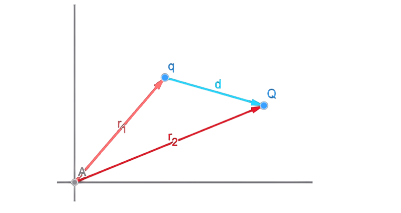
The force is inversely proportional to the square of the distance between the charges. The constant $k$ is given by the following expression, where $\varepsilon_0$ is the electric permittivity of free space:

$$k = \frac{1}{4\pi \varepsilon_0}$$

We will now define the electric field, a vector field that gives the force per unit charge:

$$\vec{F} = q\vec{E}$$ $$\vec{E} = k \frac{Q}{d^2} \hat{d}$$

We now have a simpler mathematical expression. At a distance $d$ from our reference point $\vec{r}_1$, that is, from charge $Q$, I can find the force per unit charge and multiply it by $q$ to obtain the net force on charge $q$. Let $\vec{F}_i$ be the force exerted by charge $Q_i$ on charge $q$:

$$\vec{F}_{net} = \vec{F}_1 + \vec{F}_2 + ... + \vec{F}_N$$

This is called the superposition principle. It means that the net force vector equals the sum of all the vectors. Now suppose that there are not one but many charges $Q_1, Q_2..Q_N$.

$$\vec{E} = k \sum_{i=1}^{n} \frac{Q_i}{d_i^2} \hat{d}$$

The field is found from this expression. The electric field obeys superposition. If we calculate the electric field due to every charge $Q$ in the system and add them together, we obtain the total electric field. With this formula, we can calculate the net force vector acting on charge $q$:

$$\vec{F} = q\vec{E} = kq \sum_{i=1}^{n} \frac{Q_i}{d_i^2} \hat{d}$$

Suppose that there is a continuous charge distribution. Let us denote its one-dimensional linear density by $\lambda$, its two-dimensional surface density by $\sigma$, and its three-dimensional volume density by $\rho$. By our definition of density,

$$\lambda = \frac{dq}{dx}$$ $$\sigma = \frac{dq}{dA}$$ $$\rho = \frac{dq}{dV}$$

and the total charge can therefore be calculated using

$$Q = \int dq = \int \lambda dx$$ $$Q = \int dq = \int \sigma dA$$ $$Q = \int dq = \int \rho dV$$

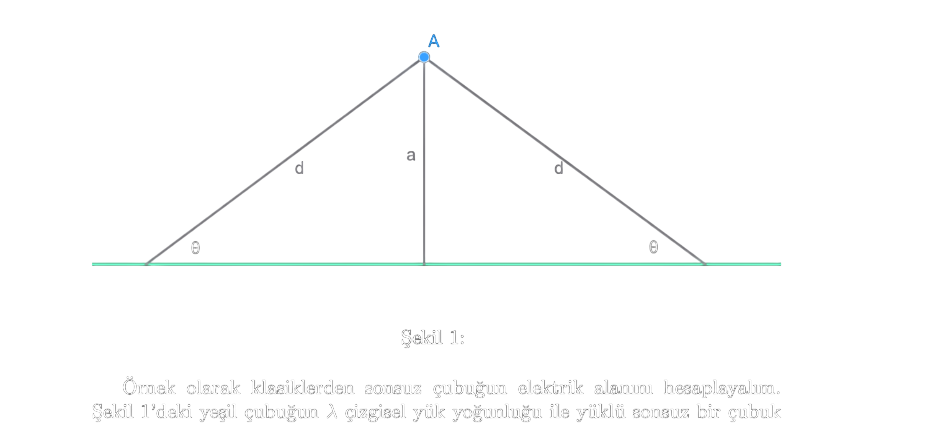
As a classic example, let us calculate the electric field of an infinite rod.
Assume that the green rod in Figure 1 is an infinite rod carrying a linear charge density $\lambda$. Let us calculate the electric field at point A, located a perpendicular distance $a$ from the rod. We know that we will find the net electric field by calculating and summing the electric fields due to every point on the rod. There is one detail to which we must now pay attention. From point A, consider points on both the right and left at a distance $d$. The horizontal components of these two points are equal in magnitude and opposite in direction. For example, the horizontal components of a point five meters to the right and a point five meters to the left cancel each other. We can therefore find the total electric field by calculating only the vertical component of every point, since the net horizontal electric field is zero. Let us call the horizontal distance $d\cos\theta$ of the point at distance $d$ by the name $x$. From the Pythagorean theorem and elementary trigonometry,

$$d^2 = a^2 + x^2$$ $$\sin\theta = \frac{a}{\sqrt{a^2 + x^2}}$$

We now know how to calculate the total charge $Q$ from the density for the electric field. We have also expressed the distance $d$ in terms of $a$ and $x$.

$$\vec{E} = k \frac{Q}{d^2} \sin\theta \, \hat{j}$$

We multiplied the electric field by $\sin\theta$ because we will calculate only its vertical component. Substituting the expressions we obtained for $d$, the sine, and $Q$ gives

$$\vec{E} = k \int_{-\infty}^{+\infty} \frac{\lambda a \, dx}{(a^2 + x^2)^{3/2}} \hat{j}$$

We know that $x = a \tan\theta$ for every point. Taking the differential gives $dx = a \sec^2\theta d\theta$, so

$$E = k\lambda \int_{-\pi/2}^{+\pi/2} \frac{a^2 \sec^2\theta}{a^3 \sec^3\theta} d\theta = \frac{k\lambda}{a} \int_{-\pi/2}^{+\pi/2} \cos\theta d\theta$$

and consequently,

$$\vec{E} = \frac{2k\lambda}{a} \hat{j} = \frac{\lambda}{2\pi \varepsilon_0 a} \hat{j}$$

Through the physics set in motion by natural philosophers who noticed something while rubbing stones together, we have calculated the electric field of an infinite rod.

Electrostatics

Electrostatics is the branch of electromagnetism that studies time-independent electric charge distributions and the electric fields they produce. The electrostatic force is conservative. In brief, this means that it is the gradient of a potential. It carries charges from high potential to low potential. We represent these forces mathematically using the following two equivalent expressions:

$$\nabla \times \vec{F} = 0$$ $$\vec{F} = -\nabla U$$

The nabla operations shown here are called the curl and gradient, respectively. $U$ is the potential-energy function. The gradient and curl vector operators are defined, respectively, as

$$\nabla = < \frac{\partial}{\partial x}, \frac{\partial}{\partial y}, \frac{\partial}{\partial z} >$$ $$\nabla f = < \frac{\partial f}{\partial x}, \frac{\partial f}{\partial y}, \frac{\partial f}{\partial z} >$$ $$\nabla \times \vec{F} = \begin{vmatrix} \hat{i} & \hat{j} & \hat{k} \\ \partial_x & \partial_y & \partial_z \\ F_x & F_y & F_z \end{vmatrix}$$ $$\nabla \times \vec{F} = (\partial_y F_z - \partial_z F_y)\hat{i} + (\partial_z F_x - \partial_x F_z)\hat{j} + (\partial_x F_y - \partial_y F_x)\hat{k}$$

Since we will use the electric field rather than force, we will use a new quantity in place of potential energy.

$$\vec{E} = -\nabla V$$

We will call $V$, the electric potential or voltage, the amount of potential energy per unit charge. For charges $q_1 \ q_2$ separated by $\vec{d}$, the potential energy between them is given by

$$U = k \frac{q_1 q_2}{|\vec{d}|}$$

and the potential energy per unit charge at the point $q$ is therefore

$$V = \frac{U}{q} = k \frac{Q}{d}$$

You might ask why, given that potential energy already exists and can be used in calculations, we go to the trouble of defining $V$ and introducing a new concept. The reason is the same as the one for defining the electric field when force already exists: it makes life easier. Suppose that we want to calculate $V$ at a point $P$ in a scenario containing $n$ charges. If $\vec{r}_i$ is the position vector of charge $q_i$, the potential $V$ at point $\vec{r}$ is found from

$$V = k \sum_i^n \frac{q_i}{|\vec{d}_i|}$$ $$\vec{d}_i = \vec{r} - \vec{r}_i$$

Multiplying this by $Q$ gives the potential energy of charge $Q$ at point $\vec{r}$. As we will see in the next part, the electric-field–potential relation offers a more elegant model than the force–potential relation. If there is a continuous charge distribution, the calculation can be performed according to those given in equation (9).

We know that the curl of a gradient is zero, and therefore, by equation (17), the curl of the electric field is also zero. Stokes' theorem for a vector field $\vec{F}$ is

$$\oint_{\partial S} \vec{F} \cdot d\vec{r} = \iint_S (\nabla \times \vec{F}) \cdot d\vec{S}$$

Thus, because the right-hand side is zero for the electric field, we know that the closed line integral on the left-hand side is zero:

$$\oint \vec{E} \cdot d\vec{r} = 0$$

This means that the line integral of the electric field around a closed path is zero. Now consider the line integral between two points. Taking $O$ as our reference, we can define the potential $V$ as

$$V(\vec{r}) = - \int_O^r \vec{E} \cdot d\vec{l}$$

and for the potential difference between two points, we can write

$$V_B - V_A = - \int_A^B \vec{E} \cdot d\vec{l}$$

We can thereby calculate and examine the concept of potential mathematically. We can now turn to Gauss's law, which is extremely valuable in electrostatics and is Maxwell's first equation. The divergence theorem for a vector field $\vec{F}$ is

$$\int_V (\nabla \cdot \vec{F}) dV = \oint_{\partial V} \vec{F} \cdot d\vec{S} = \oint_{\partial V} \vec{F} \cdot \hat{n} dS$$

To describe its intuitive meaning briefly, our vector field—think of the electric field—has lines beginning at charge $q$. If we enclose the charge or charges with a surface, these lines cross that surface. Looking at the lines perpendicular to our surface, at 90 degrees, gives us the quantity called flux. A large magnitude of flux means that the electric field is strong. Positive flux means the electric field points outward through the surface; negative flux means it points inward. This applies to any arbitrary surface we choose. For convenience, however, suppose that we now apply our formula to a sphere of radius $r$ enclosing the charges in our field. The right-hand side of the theorem is the product of the electric field and the surface area of our sphere. The resulting expression is

$$E \cdot 4\pi r^2 = \frac{1}{4\pi \varepsilon_0} \frac{Q}{r^2} 4\pi r^2 = \frac{Q}{\varepsilon_0}$$

We have obtained the integral form of Gauss's law. The other part of the divergence theorem is the integral of the divergence over the volume; since we call the amount of charge per unit volume the charge density $\rho$, the differential and integral forms of Gauss's law are

$$\nabla \cdot \vec{E} = \frac{\rho}{\varepsilon_0}$$ $$\oint_{\partial V} \vec{E} \cdot d\vec{S} = \frac{\sum Q}{\varepsilon_0}$$

Let us interpret this result. We see that the outward distribution of the electric field from a charge or charge distribution is directly proportional to the magnitude of the charge. In the integral form, we see that it depends on the net charge enclosed by the surface we choose.
Notice that the area of our chosen surface increases with the square of the distance from the charge as we move farther away. Because the electric field decreases with that same square, the divergence of the electric field depends only on the charge density. Writing the definition of divergence as

$$\nabla \cdot \vec{F} = < \frac{\partial}{\partial x}, \frac{\partial}{\partial y}, \frac{\partial}{\partial z} > \cdot < F_x, F_y, F_z > = \frac{\partial F_x}{\partial x} + \frac{\partial F_y}{\partial y} + \frac{\partial F_z}{\partial z}$$

we can see that it is, in fact, another expression of Coulomb's law. We call it Gauss's law because the mathematical divergence theorem that allows us to calculate it is attributed to Gauss. Let us now see how much this result simplifies our work. Once again, I want to calculate the electric field of an infinite rod. We said that we could choose an arbitrary surface. Let us choose a cylinder of radius $a$ and length $L$, and suppose that it encloses our infinite rod. Again, let the point we seek be located a perpendicular distance $a$ from the rod. From the integral form of Gauss's law, the product of the magnitude of the electric field and the area of our surface equals the net charge enclosed by the surface divided by $\varepsilon_0$. Let our charge density be $\lambda$. The net amount of charge inside is then $Q = \lambda L$. In applying the integral form of Gauss's law, the electric-field magnitude is constant and can therefore be taken outside the integral. The expression we obtain is the product of the electric field and the net surface area of our chosen surface. On the right-hand side, we already have an expression for the net charge in terms of the charge density:

$$E \oint dS = E 2\pi a L = \frac{\lambda L}{\varepsilon_0}$$ $$E = \frac{\lambda}{2\pi \varepsilon_0 a}$$

We found the result without having to perform a great deal of algebra and integration. Besides this practical benefit, we can also see that the electric field points toward negative charges and away from positive charges. Let us work through one more example. Suppose that there is an amount of charge $q$ in space. Let our surface be a sphere of radius $d$ enclosing this charge. Applying Gauss's law gives

$$E \cdot 4\pi d^2 = \frac{q}{\varepsilon_0}$$ $$\vec{E} = \frac{q}{4\pi \varepsilon_0 d^2} \hat{d}$$

and we have thus found the electric field at a distance $d$ from charge $q$. This is precisely the electric-field formula that we already know.

Now consider an infinite plane and let us calculate its electric field. Let the charge density of this infinite plane be $\sigma$. For Gauss's law, choose a rectangular surface that encloses the plane. Let the areas of its upper and lower faces be $A$. Because it encloses the plane, the charge contained within it is $\sigma A$. The side faces contribute nothing because the electric field of the plane is perpendicular to their area vectors, so their dot products are zero. The net contributing surface area is therefore $2A$, corresponding to the two faces of the plane. From Gauss's law,

$$E 2A = \frac{\sigma A}{\varepsilon_0}$$ $$\vec{E} = \frac{\sigma}{2\varepsilon_0} \hat{n}$$

Thus, the electric field of the infinite plane is the charge density divided by $2\varepsilon_0$. Owing to the geometry and symmetry, its direction is perpendicular to the plane.

Using equation (17) in Gauss's law, we obtain

$$\nabla \cdot \vec{E} = \nabla \cdot (-\nabla V) = -\nabla^2 V$$ $$\nabla^2 V = - \frac{\rho}{\varepsilon_0}$$

The operator acting on the potential is called the Laplacian and is calculated as

$$\nabla^2 V = \frac{\partial^2 V}{\partial x^2} + \frac{\partial^2 V}{\partial y^2} + \frac{\partial^2 V}{\partial z^2}$$

Equation (32) is called Poisson's equation. The special case in which the charge density is zero,

$$\nabla^2 V = 0$$

is called Laplace's equation. Thus, if we solve the Laplacian using the given charge density, we can find the potential and then obtain the electric field by taking the gradient of that potential. Considering that we use Maxwell's equations to determine electric and magnetic fields, equation (32), which we obtained for the potential, can provide the electrostatic electric field. We have therefore learned, for a constant charge density and a constant electric field, how to find the electric field, how to calculate the force from the electric field, how to calculate the potential, and how to calculate the electric field from the potential.

Because the Poisson and Laplace equations are partial differential equations, finding their solutions is somewhat more involved. We will discuss them in later parts.