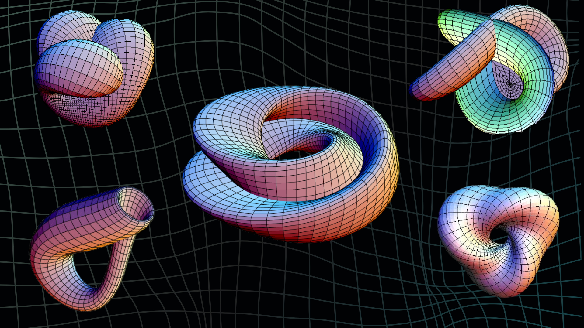
The Secrets of Surfaces: Intrinsic Metrics and Extrinsic Bending

Introduction: The Ant's and the Giant's Points of View

Hello again, everyone! If your coffee is ready, prepare to round one of the most exciting bends in differential geometry. In the previous chapter, we defined surfaces by attaching “patches” to them. But we have a problem: how can an “ant” that lives on this surface and cannot see the outside world know how far it has traveled, the sum of the interior angles of its triangles, or the size of the region it occupies?

As “giants” (observers) looking from outside, we can use our ruler to take measurements in three-dimensional space ( $\mathbb{E}^3$ ). But differential geometry is not only about looking from the outside; it is also about understanding the intrinsic character of the surface. In this chapter, we will bring together both the ant's ruler (the First Fundamental Form) and the observations of the giant looking from outside (the Second Fundamental Form).

The First Fundamental Form: Measuring Distance on a Surface

Recall that we had a surface $S$ and, at a point $p$ on it, a tangent plane $T_pS$ . The basis vectors $\mathbf{x}_u$ and $\mathbf{x}_v$ spanned this plane. If we want to calculate the length of any vector $w = a \mathbf{x}_u + b \mathbf{x}_v$ in the tangent plane, we take its inner product with itself:

|w|^2 = \langle a \mathbf{x}_u + b \mathbf{x}_v, a \mathbf{x}_u + b \mathbf{x}_v \rangle

Expanding the brackets gives Gauss's famous three coefficients:

Definition (Coefficients of the First Fundamental Form)
$E = \langle \mathbf{x}_u, \mathbf{x}_u \rangle, \quad F = \langle \mathbf{x}_u, \mathbf{x}_v \rangle, \quad G = \langle \mathbf{x}_v, \mathbf{x}_v \rangle$
These coefficients determine the geometry (metric) of the surface at that point. The squared differential length ( $ds^2$ ) on the surface is expressed by
$I_p(w) = E du^2 + 2F dudv + G dv^2$

Thanks to this formula, we can calculate arc length and area on the surface using only the parameters ( $u, v$ ) and these coefficients, without ever involving the $x, y, z$ coordinates. This is called intrinsic geometry.

A Surprising Result: A Cylinder Is Actually Flat!

We now come to the mind-bending part: the “counterexamples.” We will consider two different surfaces and listen to what their First Fundamental Forms have to tell us.

The Plane (Our Reference Point)

Parametrize the plane by $\mathbf{x}(u, v) = (u, v, 0)$ .

$\mathbf{x}_u = (1, 0, 0) \implies E = 1$
$\mathbf{x}_v = (0, 1, 0) \implies G = 1$
$\mathbf{x}_u \cdot \mathbf{x}_v = 0 \implies F = 0$

Metric: $ds^2 = du^2 + dv^2$ (the familiar Pythagorean theorem!)

The Cylinder (A Counterintuitive Example)

Consider a cylinder of radius 1: $\mathbf{x}(u, v) = (\cos u, \sin u, v)$ .

$\mathbf{x}_u = (-\sin u, \cos u, 0) \implies E = \sin^2 u + \cos^2 u = 1$
$\mathbf{x}_v = (0, 0, 1) \implies G = 1$
$F = 0$

Metric: $ds^2 = du^2 + dv^2$

WAIT A MINUTE! The First Fundamental Forms of the plane and the cylinder are THE SAME!
This means that in terms of intrinsic geometry, there is NO difference between the cylinder and the plane. Put one ant on the cylinder and another on a table. If each draws triangles, both will find that the interior angles sum to 180 degrees. A cylinder may be bent, but it is not intrinsically curved. You can bend a sheet of paper into a roll (a cylinder), but you cannot turn it into a sphere without tearing it.

The Sphere (True Curvature and the Cartographer's Ordeal)

Things change on a sphere of radius $R$ : $\mathbf{x}(u, v) = (R \sin u \cos v, R \sin u \sin v, R \cos u)$ .
A calculation gives $E=R^2, F=0$ , but $G=R^2 \sin^2 u$ .
The coefficients vary with position ( $u$ )! This is why planar geometry does not work here. You cannot unfold the sphere onto a plane without distorting distances.

The Second Fundamental Form: The External View and Bending

We have seen that the cylinder and the plane are intrinsically the same. But we have eyes: the cylinder bends through space! To understand this difference in “bending,” we must step outside the surface and examine how its normal vector ( $N$ ) changes.

If we take the second-order derivatives of the surface ( $\mathbf{x}_{uu}, \mathbf{x}_{uv}, \mathbf{x}_{vv}$ ) and project them onto the unit normal ( $N$ ), we find “how far the surface departs from its tangent plane” in the given direction.

Definition (Coefficients of the Second Fundamental Form)
$L = \langle \mathbf{x}_{uu}, N \rangle, \quad M = \langle \mathbf{x}_{uv} N \rangle,$ $N_c = \langle \mathbf{x}_{vv}, N \rangle$

Now let us return to the cylinder and the plane:

Plane: All second derivatives are 0. Hence $L=M=N_c=0$ . The plane does not bend.
Cylinder: The vector $\mathbf{x}_{uu} = (-\cos u, -\sin u, 0)$ is nonzero and points in the same direction as the normal vector. Therefore $L \neq 0$ .

There is the difference! The Second Fundamental Form detects the shape of the surface in ambient space ( $\mathbb{E}^3$ ) and how it bends. We will gradually begin discussing Gaussian curvature, but first let us take a visual look at the famous hyperbolic paraboloid, better known as the Pringles chip. This shape will show the orientation of the normal vectors and thus provide a fine introduction to curvature.

An Example: The Hyperbolic Paraboloid (Saddle Surface)

One of the finest examples of bending is the hyperbolic paraboloid, shaped like a “saddle” or a “Pringles chip.” Its equation is $z = x^2 - y^2$ , or parametrically $\mathbf{x}(u,v) = (u, v, u^2-v^2)$ .

Imagine moving over this surface. It curves upward in one direction and downward in the other. This contrast manifests itself in the behavior of the normal vectors.

The Python code below plots the surface and its normal vectors. Notice how the normals spread in different directions; this shouts to us that the surface has “negative curvature.”

import numpy as np  
import matplotlib.pyplot as plt  
from mpl_toolkits.mplot3d import Axes3D  
  
fig = plt.figure(figsize=(10, 8))  
ax = fig.add_subplot(111, projection='3d')  
  
# Semer Yuzeyi: z = x^2 - y^2  
u = np.linspace(-1, 1, 15)  
v = np.linspace(-1, 1, 15)  
U, V = np.meshgrid(u, v)  
X, Y = U, V  
Z = U**2 - V**2  
  
ax.plot_surface(X, Y, Z, cmap='viridis', alpha=0.7)  
  
# Normallerin Hesabi ve Cizimi  
# xu = (1,0,2u), xv = (0,1,-2v) -> Normal ~ (-2u, 2v, 1)  
u_sample = np.linspace(-0.8, 0.8, 6)  
v_sample = np.linspace(-0.8, 0.8, 6)  
Us, Vs = np.meshgrid(u_sample, v_sample)  
Zs = Us**2 - Vs**2  
  
Nx = -2 * Us  
Ny = 2 * Vs  
Nz = np.ones_like(Us)  
Norm = np.sqrt(Nx**2 + Ny**2 + Nz**2) # Birimlendirme  
  
ax.quiver(Us, Vs, Zs, Nx/Norm, Ny/Norm, Nz/Norm, length=0.3, color='red')  
ax.set_title("Hiperbolik Paraboloid ve Normal Vektorleri")  
plt.show()

Hyperbolic Paraboloid and Normal Vectors.

A Preview of the Grand Finale: Curvature

We have two forms at our disposal:

$I$ : Intrinsic measurement (the metric)
$II$ : Extrinsic bending (the shape)

The ratio of the two gives us differential geometry's most sacred concept, Gaussian curvature ( $K$ ).

K = \frac{\det(II)}{\det(I)} = \frac{LN_c - M^2}{EG - F^2}

What is fascinating about this formula is that, although $L, M, N_c$ require an external point of view, Gauss's Theorema Egregium (Remarkable Theorem) proves that $K$ can also be calculated solely in terms of $E, F, G$ . The curvature of a surface is therefore its destiny: bending cannot change it!

$K > 0$ : Sphere (closed and convex)
$K < 0$ : Saddle / hyperbolic (saddle-shaped)
$K = 0$ : Plane or cylinder (planar geometry applies)

Using Python to Investigate Metrics and Bending

The code below performs both an intrinsic ( $E,F,G$ ) and an extrinsic ( $L,M,N_c$ ) analysis of any surface you provide.

import sympy as sp

u, v = sp.symbols('u v', real=True)
R = sp.symbols('R', real=True)

# Ornek: Kure Yuzeyi
surf = [R * sp.sin(u) * sp.cos(v), 
        R * sp.sin(u) * sp.sin(v), 
        R * sp.cos(u)]

def analyze_surface(pos, u, v):
    # 1. Kisim: Tegetler ve Birinci Form
    xu = [sp.diff(i, u) for i in pos]
    xv = [sp.diff(i, v) for i in pos]
    
    E = sp.simplify(sum(i*i for i in xu))
    F = sp.simplify(sum(i*j for i,j in zip(xu, xv)))
    G = sp.simplify(sum(j*j for j in xv))
    
    # 2. Kisim: Normal ve Ikinci Form
    # Normal vektor (Cross Product)
    n_raw = [xu[1]*xv[2]-xu[2]*xv[1], xu[2]*xv[0]-xu[0]*xv[2], xu[0]*xv[1]-xu[1]*xv[0]]
    n_mag = sp.sqrt(sum(k*k for k in n_raw))
    N = [k/n_mag for k in n_raw] # Birim Normal
    
    xuu = [sp.diff(i, u) for i in xu]
    xuv = [sp.diff(i, v) for i in xu]
    xvv = [sp.diff(i, v) for i in xv]
    
    L = sp.simplify(sum(i*j for i,j in zip(xuu, N)))
    M = sp.simplify(sum(i*j for i,j in zip(xuv, N)))
    Nc = sp.simplify(sum(i*j for i,j in zip(xvv, N)))
    
    return (E, F, G), (L, M, Nc)

# Hesapla
(E, F, G), (L, M, Nc) = analyze_surface(surf, u, v)

print(f"I. Form: E={E}, F={F}, G={G}")
print(f"II. Form: L={L}, M={M}, N={Nc}")

In the Next Chapter...

We now have both our ruler and our bending gauge. In the next chapter, we will delve into the concept of curvature ( $K$ ), prove why maps always misrepresent the world, and tip our hats to Gauss's genius.

Stay with mathematics—and with curves!