Differential Geometry Series Part 8

Surface Theory: Smoothness, Pitfalls, and the Real World

Greetings! Welcome to Chapter 8 of our differential geometry series. In earlier chapters, we chased one-dimensional curves and took the bends with the Frenet frame. Now we are moving up a dimension. From here on, we will study structures that we can walk on, draw maps upon, and even spill coffee over: surfaces.

Be warned, however: surfaces are more temperamental than curves. Not every graph $f(x,y)$ is our friend. In this chapter, we will both meet our friends and expose the structures that “look like surfaces but are actually trouble.”

What Is a Surface? (A Little More Formality)

Imagine a set floating in space. When do we call it a “regular surface”? As mathematicians, we cannot simply say, “It looks nice.” We need a sturdier definition.

Definition (Regular Surface)

Let $S \subset \mathbb{E}^3$ be a subset. If, for every point $p \in S$, there is a neighborhood $V \subset S$ containing $p$ and a map $\mathbf{x}: U \rightarrow V$ from an open set $U \subset \mathbb{R}^2$ to $V$, and this map satisfies the following three conditions, then $S$ is called a regular surface:

1. Differentiability: The function $\mathbf{x}$ has continuous partial derivatives of every order. (In other words, there are no sudden breaks or sharp corners in the surface; it is smooth as butter.)
2. Homeomorphism: $\mathbf{x}$ must be one-to-one and onto, and its inverse must also be continuous. (The surface must not fold over or knot into itself. You may crumple a sheet of paper into a ball, but you cannot tear it and pass it through itself.)
3. Regularity Condition: For every $(u,v) \in U$, the differential map must be one-to-one. In practice, this means

$$\mathbf{x}_u \wedge \mathbf{x}_v \neq \mathbf{0}$$

This third condition is vital. The vectors $\mathbf{x}_u$ and $\mathbf{x}_v$ span the “tangent plane” of the surface at that point. If their cross product is zero, then either one of the vectors is zero or they are parallel. In that case, no plane is formed there; the surface “contracts” or “comes to a point.”

Counterexamples: Where Do Things Go Wrong?

Not every shape we see is a surface. To understand why the conditions in the definition are necessary, let us examine “broken” examples—that is, counterexamples.

Example A: The Cone (The Pointed-Tip Problem)

Think of an ordinary ice-cream cone. Mathematically, it is given by the equation $z = \sqrt{x^2 + y^2}$. We can parametrize it as follows:

$$\mathbf{x}(u, v) = (u \cos v, u \sin v, u)$$

Here, $u$ is the radius ($u \ge 0$), while $v$ is the angle.

Let us look at the derivatives:

• $\mathbf{x}_u = (\cos v, \sin v, 1)$
• $\mathbf{x}_v = (-u \sin v, u \cos v, 0)$

Now calculate the cross product:

$$\mathbf{x}_u \wedge \mathbf{x}_v = (-u \cos v, -u \sin v, u)$$

The length (norm) of this vector is

$$\sqrt{u^2 \cos^2 v + u^2 \sin^2 v + u^2} = \sqrt{2u^2} = u\sqrt{2}$$

Take care! If $u = 0$—that is, if we are at the very apex of the cone—the norm is zero!

$$\mathbf{x}_u \wedge \mathbf{x}_v = \mathbf{0}$$

This means that we cannot define a tangent plane at the apex of the cone. That point is “sharp.” The cone is therefore a regular surface everywhere except its apex, but it is not a regular surface if the apex is included. Differential geometry does not care for that pointed tip.

Example B: Self-Intersecting Surfaces

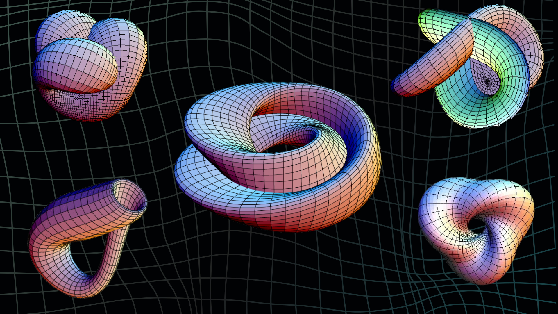
If our map is not one-to-one—violating condition 2 of the definition—the surface passes through itself. The Klein bottle, for example, cannot be drawn in three-dimensional space without self-intersection; it requires four dimensions. If you try to draw it in three dimensions, it must intersect itself somewhere. At a point of self-intersection, there are “two” tangent planes, which conflicts with our notion of a function.

Applications: Where Is This Mathematics Used?

You might say, “Professor, this is all well and good, but I can already see that the tip of a cone is sharp. Why do we need derivatives?” Fair enough, but this theory has a very broad range of applications.

Application 1: Computer Graphics and Game Engines

The faces of characters and the body panels of cars in the high-resolution games you play are really “surface patches” (Bézier surfaces or NURBS). To calculate how light reflects from such a surface, the game engine needs the normal vector ($N$).

$$N = \frac{\mathbf{x}_u \wedge \mathbf{x}_v}{||\mathbf{x}_u \wedge \mathbf{x}_v||}$$

If your model has a “sharp” point like the cone and you have not defined it properly in mathematical terms, the game engine cannot calculate the normal vector there (it encounters division by zero), and the lighting “breaks” at that point—you see black spots or strange glare.

Application 2: Cartography

The Earth is round—approximately spherical—while paper is flat. Mapping the surface of a sphere (a surface in $\mathbb{E}^3$) onto a plane ($\mathbb{R}^2$) is what we call the inverse of a parametrization.

Differential geometry tells us that the “curvature” of a sphere—Gaussian curvature, which we will meet later—is positive, whereas the curvature of a plane is zero. It is therefore impossible to map the sphere onto the plane without distorting distances or angles. In other words, all your maps are lying to you! They either make Greenland look enormous, as the Mercator projection does, or distort shapes. This is a mathematical necessity.

Comparing “Broken” and “Regular” Surfaces with Python

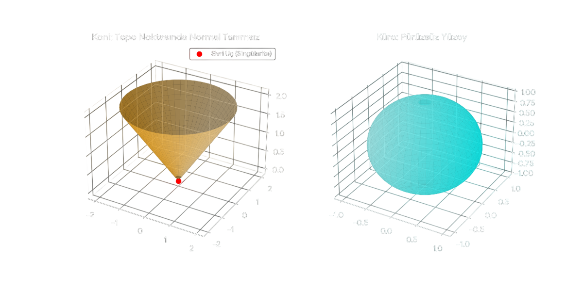
Visualizing the theoretical notion of “regularity” is crucial to understanding it. Let us consider a sphere and a cone. A sphere is smooth at every point, and a unique normal vector—an arrow perpendicular to the surface—can be defined everywhere.

At the apex $(0,0,0)$ of the cone, however, things become complicated. The surface “comes to a point,” and mathematically the condition $\mathbf{x}_u \times \mathbf{x}_v = 0$ occurs. The tangent plane cannot be defined at the apex of the cone; this is therefore a singular point.

The Python code below visualizes the fundamental difference between these two surfaces:

import numpy as np
import matplotlib.pyplot as plt

fig = plt.figure(figsize=(12, 6))

# --- KONI: Reguler olmayan nokta barındırır ---
u = np.linspace(0, 2*np.pi, 50)
v = np.linspace(0, 2, 20)
U, V = np.meshgrid(u, v)
X = V * np.cos(U); Y = V * np.sin(U); Z = V

ax1 = fig.add_subplot(121, projection='3d')
ax1.plot_surface(X, Y, Z, color='orange', alpha=0.6)
ax1.set_title("Koni: Tepe Noktası Problemlidir")
ax1.set_box_aspect((1, 1, 1)) # Ölcek duzeltme

# --- KURE: Her noktada regulerdir ---
v_s = np.linspace(0, np.pi, 30)
U_s, V_s = np.meshgrid(u, v_s)
X_s = np.sin(V_s) * np.cos(U_s); Y_s = np.sin(V_s) * np.sin(U_s); Z_s = np.cos(V_s)

ax2 = fig.add_subplot(122, projection='3d')
ax2.plot_surface(X_s, Y_s, Z_s, color='cyan', alpha=0.6)
ax2.set_title("Kure: Puruzsuz ve Reguler")
ax2.set_box_aspect((1, 1, 1))

plt.show()

Conclusion

As we can see, if we want to do differential geometry, our surface must be “smooth”—at least in the region where we are working. In the next chapter, we will learn how to make measurements on these smooth surfaces using the First Fundamental Form.