Differential Geometry Series Part 7

Differential Geometry Series, Chapter 7: The Art of Sniffing Out a Curve

Introduction: What's on the Menu?

Hello, everyone. In the previous article, we put pen to paper on curvature and torsion, the two most fundamental concepts of the Frenet frame. In this article, we will try to understand the structure of a curve through its curvature and torsion.

A Twisty-Turny Curve!

This chapter will really be more of a worked example than a chapter. Consider a curve $\alpha$ whose curvature $\kappa$ and torsion $\tau$ satisfy $\frac{\kappa}{\tau}=sbt\neq 0, \forall s$. By the fundamental theorem of curves, such a curve exists. Can we classify it explicitly? Let us suppose that our constant equals $\tan\theta$ for some angle $\theta$. Our motivation for this assumption is that the tangent function is surjective.

Then $\kappa\cos\theta-\tau\sin\theta=0$. Thus, for the normal vector $\mathbf{N}$ of the curve $\alpha$, $(\kappa\cos\theta-\tau\sin\theta)\mathbf{N}=0$. Why bring the normal vector into it? Because multiplying curvature and torsion by the normal vector gives us, respectively, derivatives of the tangent and binormal vectors. That gives us a way forward. The equation we have just written can therefore be expressed as

$$\cos\theta\ \mathbf{T}'+\sin\theta \ \mathbf{B}'= 0$$

which allows us to define the unit vector

$$u:=\cos\theta \ \mathbf{T}+\sin\theta\ \mathbf{B}$$

This vector makes a constant angle $\theta$ with $\mathbf{T}$. We know—or, if we did not, we do now—that a curve whose tangent makes a constant angle with a fixed direction is called a helix. We may therefore say that curves for which the ratio between curvature and torsion is a nonzero constant are helices. Below is the Python version of what we have done.

import numpy as np
import matplotlib.pyplot as plt
from mpl_toolkits.mplot3d import Axes3D

def helix(theta, t_range=np.linspace(0, 10, 500)):  
    kappa = np.cos(theta)
    tau = np.sin(theta)  # Burulma
    x = np.cos(kappa * t_range)
    y = np.sin(kappa * t_range)
    z = tau * t_range
    return x, y, z

thetas = np.linspace(0, np.pi/2, 5)
fig = plt.figure(figsize=(10, 8))
ax = fig.add_subplot(111, projection='3d')

for theta in thetas:
    x, y, z = helix(theta)
    ax.plot(x, y, z, label=f"theta={np.degrees(theta):.0f}")

ax.set_xlabel("X")
ax.set_ylabel("Y")
ax.set_zlabel("Z")
ax.legend()
ax.set_title("Farkli Theta Acilari icin Helis Egrileri")
plt.show()

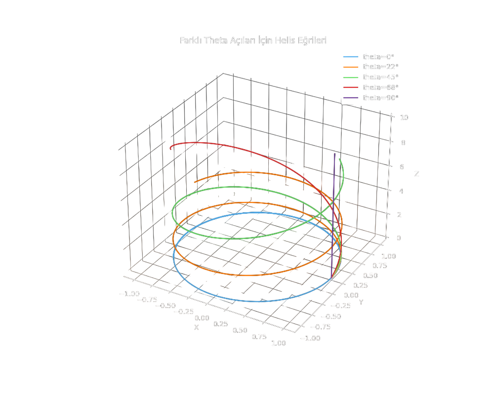
I will leave the cases where the angle is zero or a right angle for you to interpret. Meanwhile, let us continue. As you can see, a relation between curvature and torsion alone can tell us what a curve is. Let us proceed to our next example.

Example

Once again, consider a planar curve of constant curvature in our three-dimensional Euclidean space (did I mention that we will be hanging around in this space until further notice? If not, consider it said). Thus $\tau=0$. We can immediately say that this curve is not a helix, but what is it? Let us write down the Frenet frame.

$$\begin{bmatrix}\textbf{T}'\\\textbf{N}'\\\textbf{B}'\end{bmatrix} = \begin{bmatrix}0 & \kappa & 0 \\-\kappa& 0& 0 \\ 0& 0& 0\end{bmatrix} \begin{bmatrix}\textbf{T}\\\textbf{N}\\\textbf{B}\end{bmatrix}$$

Taking into account that $\kappa$ is constant, we obtain $\textbf{B}=\textbf{B}_0$, a constant vector, and $\textbf{T}''=-\kappa^2\textbf{T}$. At this point, the road forks. If $\kappa=0$, our curve $\alpha$ is a straight line. If $\kappa\neq 0$, however, we can see that the tangent vector is a regular haunt of sines and cosines. This suggests that the curve is a circle. In fact, that is more than a conjecture: solve the equation and substitute the result into the equation for the normal vector, and you will see that our curve really is a circle, with radius $\frac{1}{\kappa}$. You may remember that I discussed the osculating circle in earlier chapters. This is where you are supposed to say “wow,” just so you know...

The moral of the story is that you can find a curve directly from its tangent and torsion. You may need to solve a differential equation or two, but you will find it in the end. Let us now begin our closing remarks on curves by discussing their indicatrices and evolutes.

Definition (Tangent indicatrix)

Let $\alpha:I\rightarrow\mathbb{R}^3$ be a regular curve parametrized by arc length, and let $\textbf{T}_\alpha(s)$ be its tangent at $s$. The curve $\beta:I\rightarrow\mathbb{R}^3$ defined by $\beta(s):=\textbf{T}_\alpha(s)$ is called the tangent indicatrix of the curve.

Definition (Normal indicatrix)

Let $\alpha:I\rightarrow\mathbb{R}^3$ be a regular curve parametrized by arc length, and let $\textbf{N}_\alpha(s)$ be its normal at $s$. The curve $\gamma:I\rightarrow\mathbb{R}^3$ defined by $\gamma(s):=\textbf{N}_\alpha(s)$ is called the normal indicatrix of the curve.

Definition (Binormal indicatrix)

Let $\alpha:I\rightarrow\mathbb{R}^3$ be a regular curve parametrized by arc length, and let $\textbf{B}_\alpha(s)$ be its binormal at $s$. The curve $\mu:I\rightarrow\mathbb{R}^3$ defined by $\mu(s):=\textbf{B}_\alpha(s)$ is called the binormal indicatrix of the curve.

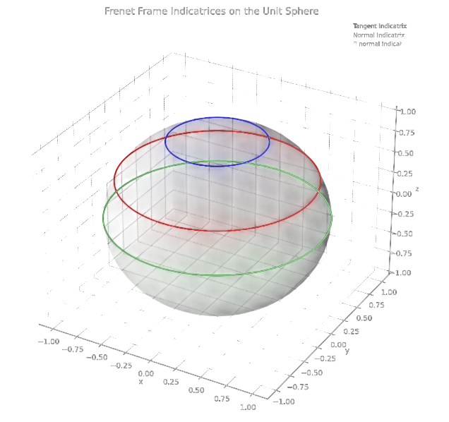
Many sources call the objects defined above “spherical indicatrices.” The reason is that all the indicatrices are unit vectors and must ultimately live on a sphere. Let us now turn to the theorem giving the Frenet frame of the tangent indicatrix, the one we encounter most often.

Theorem

Let $\alpha:I\rightarrow\mathbb{R}^3$ be a regular curve parametrized by arc length, and let $\beta:I\rightarrow\mathbb{R}^3$ be its tangent indicatrix. The tangent, normal, and binormal vectors of $\beta$, together with its curvature and torsion, are as follows.

$$\begin{aligned} \textbf{T}_\beta&=\textbf{N}_\alpha \\ \textbf{N}_\beta&=-\frac{\kappa_\alpha\textbf{T}_\alpha+\tau_\alpha\textbf{N}_\alpha}{\sqrt{\kappa_\alpha^2+\tau_\alpha^2}}\\ \textbf{B}_\beta&=\frac{\kappa_\alpha\textbf{B}_\alpha-\tau_\alpha\textbf{T}_\alpha}{\sqrt{\kappa_\alpha^2+\tau_\alpha^2}}\\ \kappa_\beta &=\frac{\kappa_\alpha^2+\tau_\alpha^2}{\kappa_\alpha^2}\\ \tau_\beta &=\frac{\kappa_\alpha\tau_\alpha'-\kappa_\alpha'\tau_\alpha}{\kappa_\alpha(\kappa_\alpha^2+\tau_\alpha^2)} \end{aligned}$$

Lemma

The tangent indicatrix of a planar curve is the unit circle.

Example

The curve $\alpha(t)=(\cos t,\sin t, t)$ is a helix (prove it). Its tangent, normal, and binormal indicatrices are shown below.

The Evolute of a Curve

Here is another term I have never quite managed to render in Turkish. As usual, take a beautiful curve $\alpha$. We know that, for a given $s$, its radius of curvature is $\frac{1}{\kappa(s)}$. Where there is a radius, there is naturally a circle; our present aim is to find the center of that circle in local coordinates. Consider the Frenet frame. We defined the normal vector as the unit vector indicating the direction of $\textbf{T}'$, and we know it is perpendicular to the tangent. We also know that the direction of $\textbf{T}'$ changes according to the sign of the curvature. It follows that $\textbf{N}$ points toward the center of the osculating circle. Starting from our current point $\alpha(s)$ and moving a distance $\frac{1}{\kappa(s)}$ in the normal direction therefore takes us to the center of that circle. The set of the centers of these osculating circles, over all $s$, is what we call the evolute. Now you see why I could not translate it into Turkish, right? Let us move on to the definition.

Definition (Evolute)

Let $\alpha:I\rightarrow \mathbb{R}^3$ be a regular curve parametrized by arc length. The curve $\beta:I\rightarrow \mathbb{R}^3$ defined by

$$\beta(s)=\alpha(s)+\frac{1}{\kappa(s)}\textbf{N}(s)$$

is called the evolute of $\alpha$.

We will now look at the evolutes of several familiar curves.

Example

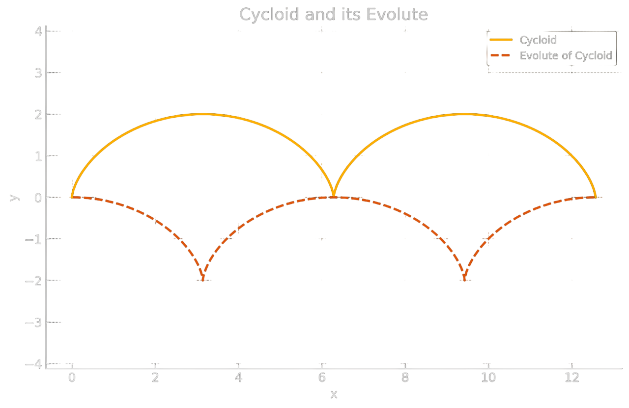
The concept of an evolute is actually much older than modern differential geometry. As far back as the time of Apollonius, conic sections were fashionable in Ancient Greece. With the geometric knowledge then available, they were the most complicated curves one could study. We will soon see that evolutes suit conic sections particularly well. The concept first became widely discussed, however, in connection with the famous pendulum and tautochrone problem. What I really want to do in this example is show how the concept relates to pendulums and to finding the tautochrone curve. A cycloid is the curve parametrized by $x=r(\theta-\sin\theta)$ and $y=r(1-\cos\theta)$, where $r$ is constant. For simplicity, take $r=1$. The curvature of this curve is

$$\kappa(\theta)=\frac{\cos\theta-1}{(2-2\cos\theta)^{3/2}}$$

From here, you can readily calculate the normal vector—you with pencil and paper, I with Python. In the end, the parametric equation of the evolute is $x=\theta+\sin\theta$, $y=\cos\theta-1$, which is nothing other than a translated cycloid. Thus:

Theorem

If $\alpha$ is a cycloid, then its evolute is also a cycloid.

The image below visualizes the example above.

Example

If $\alpha$ is a circle, its evolute consists of a single point. Instead of explaining the reason directly, I will give you a hint: look at the informal definition of the evolute.

Example

Now consider a helix. The evolute of a helix is again a helix, but with a different orientation. Think of two arcs whose ends point in opposite directions. Below you can see the helix $\alpha(s)=(\cos s,\sin s, s)$ and the graph of its evolute.

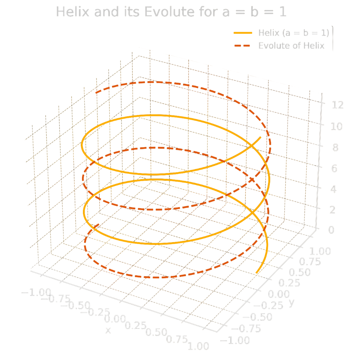
We could extend these examples much further, but I think the subject is clear. In this chapter, we played at identifying curves from their curvature and torsion, then derived new curves from a curve's curvature and the other elements of its Frenet frame. As you can see, curves are a boundless sea: no matter how long you swim, you never reach the end. That is all from us for this chapter. The next will be a bit of a surprise, because I will either move on to surfaces in Euclidean space or begin looking at curves in Minkowski space. Stay well!