The Frenet Frame

Hello, everyone! I hope all is well. In the fifth chapter of our journey through differential geometry, I have a great deal to add to the concept of a curve defined in the previous chapters. Enjoy the article.

The Frenet Frame of a Curve in Three-Dimensional Euclidean Space

In this section, we will build new concepts on top of the tangent introduced in the previous chapter.

Theorem

Let $T(s)$ be the unit tangent curve of $\alpha : I \to E^{3}$. Then $T(s) \perp \dfrac{dT}{ds}$.

Proof.

This is actually very easy. Since $\langle T(s), T(s)\rangle = 1$, differentiating both sides with respect to $s$ gives $\left\langle T(s), \dfrac{dT}{ds}\right\rangle = 0$, from which orthogonality follows. □

This theorem is simple but powerful, because it points to the existence of another vector field perpendicular to the tangent of a curve. This vector field is parallel to the derivative of the tangent and is called the unit normal of the curve.

Definition

Let $T(s)$ be the unit tangent curve of $\alpha : I \to E^{3}$.

$$N(s)=\frac{\dfrac{dT}{ds}}{\left\|\dfrac{dT}{ds}\right\|}$$

The curve defined above is called the unit normal of $\alpha$.

The definition makes it clear that the unit normal is parallel to the derivative of the tangent. There is another point I want to emphasize, however. The norm of the derivative of the tangent gives us important information: as the length along the curve changes, the tangent changes with it, and this norm measures the magnitude of that change. We call it the curvature of the curve.

Definition

Let $T(s)$ be the unit tangent curve of $\alpha : I \to E^{3}$. The curvature $\kappa(s)$ of this curve is defined by

$$\kappa(s)=\left\langle \frac{dT}{ds}, N \right\rangle$$

Corollary

Let $T(s)$ be the unit tangent, $\kappa(s)$ the curvature, and $N(s)$ the unit normal curve of $\alpha : I \to E^{3}$. Then the following equalities hold.

$$\frac{dT}{ds}=\kappa N$$ $$|\kappa(s)|=\left\|\frac{d^{2}\alpha}{ds^{2}}\right\|$$

Regrettably, the arc-length parameter is not something that will always be handed to you, so you may need other methods to calculate curvature. For that reason, after introducing the binormal vector field and torsion, I will give you another formula and prove it. In any case, let us continue our voyage of discovery. Given a curve, we can find a vector field tangent to it and another vector field normal to it at every point; what is more, we know its curvature. What we now want is to construct a local basis for the curve. Here is what I mean. In three-dimensional space, what does a point $P(x,y,z)$ signify? It means that its component along the $x$-axis is $x$, its component along the $y$-axis is $y$, and its component along the $z$-axis is $z$. Our axes therefore form a basis. In the same way, we want to express a point relative to a special coordinate system that we calculate at a point $s$ on a curve $\alpha$ (that sentence became rather like saying, “Of course you vehemently oppose entrusting children, placed in your care by their mothers, to a woman you consider inadequate in every respect”). Can we calculate a point using $T$ and $N$? The answer is “not always,” because our space is three-dimensional, and we cannot span a three-dimensional space with two vectors (recall the notion of spanning from linear algebra). We therefore need one more vector; then our local—yes, local—basis will be ready.

The Missing Piece: The Binormal Vector!

Let us do something quite different and differentiate the normal. In fact, to keep the calculus crowd from weeping, let me use more formal language: “Let the curve $\alpha : I \to E^{3}$ have the arc-length parameter $s$, tangent $T$, and normal $N$.” Then}

$$\frac{dN}{ds}$$

How do we calculate this? We will behave like physicists and imagine some vectors as we work, just so you know. Let us begin. Since $\langle N, N\rangle = 1$,

$$\frac{d}{ds}\langle N, N\rangle = 2\left\langle \frac{dN}{ds}, N \right\rangle = 0$$

and it follows that $N \perp \frac{dN}{ds}$. One might initially—and mistakenly—conclude that $\frac{dN}{ds} // T$, but we know that

$$N=\frac{1}{\kappa}\frac{dT}{ds}$$

Differentiating this gives

$$\frac{dN}{ds} = -\frac{\kappa'}{\kappa^{2}}\frac{dT}{ds} +\frac{1}{\kappa}\frac{d^{2}T}{ds^{2}}$$

I can almost hear you asking what this is supposed to yield. Here it is: we know that $\frac{dT}{ds}$ is perpendicular to the tangent. Because the derivative of the normal contains this vector among its components—that is, because it has a component perpendicular to the tangent—the derivative of the normal cannot be parallel to the tangent. Besides the tangent vector, then, it must contain another component perpendicular to both the normal and the tangent. We call this vector the binormal vector, denoted by $B$. To summarize the discussion so far, the derivative of the normal can be written, for functions $f(s)$ and $g(s)$, as

$$\frac{dN}{ds}=f(s)T+g(s)B$$

Let us now examine $f(s)$ and $g(s)$. By the definition of the binormal vector, we know that $T \perp B$ and $N \perp B$. Indeed, by declaring that the binormal should be a unit vector (I have very good reasons for this), we may write $B = T \times N$. Using this and taking the inner product of both sides of the equation above with $T$, we obtain

$$\left\langle \frac{dN}{ds}, T \right\rangle=f(s)$$

The left-hand side is not entirely unfamiliar. When defining curvature, we observed that $\left\langle \frac{dT}{ds}, N \right\rangle=\kappa$. Moreover, since $T \perp N$,

$$\frac{d}{ds}\langle N, T\rangle = \left\langle \frac{dT}{ds}, N \right\rangle + \left\langle \frac{dN}{ds}, T \right\rangle = 0$$

Combining the two equations gives

$$f(s)=-\kappa(s)$$

So curvature has appeared once again. On the other hand, using orthogonality in a similar way,

$$\left\langle \frac{dB}{ds}, N\right\rangle = -\left\langle \frac{dN}{ds}, B\right\rangle$$

and therefore

$$g(s)=-\left\langle \frac{dB}{ds}, N\right\rangle$$

What is this expression? Torsion itself. The torsion of a curve is denoted by $\tau(s)$, so $g(s)=\tau(s)$. With our calculations complete for now, let us turn to the results.

Corollary

1. $\left\langle \dfrac{dB}{ds}, N\right\rangle = -\tau(s)$
2. $\dfrac{dN}{ds} = -\kappa T + \tau B$

I want to look a little more closely at the first result. We agree that the component of the derivative of the binormal in the normal direction is $-\tau$. Does it have any other component? Because the binormal is also defined as a unit vector, we know that $\left\langle \dfrac{dB}{ds}, B\right\rangle = 0$, so there is no component in the binormal direction. Is there one in the tangent direction? To see, use the definition $B = T \times N$. Differentiating, we obtain

$$\frac{dB}{ds}=T\times N'$$

This tells us that the derivative of the binormal is perpendicular to the tangent, so it has only a normal component. Hence we obtain the following result.

Corollary

$$\frac{dB}{ds}=-\tau\cdot N$$ $$\frac{dN}{ds}=\kappa(s)T+\tau(s)B$$

We now have three mutually perpendicular, and therefore linearly independent, vectors, and they span three-dimensional Euclidean space. Every vector can thus be written as a linear combination of these three vectors, so they form a local basis for every $s$. This is what we call the Frenet frame.

The Frenet Frame of a Curve

Definition

Let the curve $\alpha : I \to E^{3}$ have arc-length parameter $s$. Let its curvature be $\kappa(s)$, its torsion $\tau(s)$, its tangent $T(s)$, its normal $N(s)$, and its binormal $B(s)$. Then the Frenet frame of this curve is

$$\{\kappa(s), \tau(s), T(s), N(s), B(s)\}$$

The elements of the Frenet frame are found by solving the following system of differential equations:

$$\begin{bmatrix} T'\\ N'\\ B' \end{bmatrix} = \begin{bmatrix} 0 & \kappa & 0\\ -\kappa & 0 & \tau\\ 0 & -\tau & 0 \end{bmatrix} \begin{bmatrix} T\\ N\\ B \end{bmatrix}$$

Readers who have previously taken a differential equations course will be accustomed to systems of this kind. Although this is actually a rather elementary system of differential equations, solving it gives us the entire curve. In other words, when the curvature and torsion functions are given, solving this system yields a curve. That means that the curvature and torsion of a curve are specific to that curve; no other curve has the same properties. This statement gives us the fundamental theorem of curves in Euclidean space.

The Fundamental Theorem of Curves in Euclidean Space

Let differentiable functions $\kappa(s) > 0$ and $\tau(s)$ be given. Then there exists only one regular curve $\alpha : I \to E^{3}$ parametrized by arc length $s$ whose curvature is $\kappa(s)$ and whose torsion is $\tau(s)$. Other curves are rotations or translations of this curve; that is, they are congruent to it.
We will omit the proof because it concerns differential equations rather than differential geometry. The theorem is in fact an application of the existence and uniqueness theorem. As I mentioned earlier, life is not always full of delights: sometimes a curve may not have an arc-length parametrization (see the example below). In such cases, calculating the Frenet frame can be a little more laborious, though certainly not impossible.

Example

Let the curve $\alpha : (0,1) \to E^{3}$ be defined by $\alpha(t) = (t, t^{2}, \sin t)$. Its arc-length parameter is calculated as

$$s(t) = \int_{0}^{t}\|\alpha'(\eta)\|d\eta = \int_{0}^{t}\sqrt{1+4\eta^{2}+\cos^{2}\eta}\, d\eta$$

But this integral has no elementary antiderivative and can only be approximated numerically (try it if you do not believe us).

Theorem

Let $\alpha : I \to E^{3}$ be a curve with an arbitrary parameter $t$. Its curvature $\kappa(t)$, torsion $\tau(t)$, tangent $T(t)$, normal $N(t)$, and binormal $B(t)$ are found by solving the following system of differential equations.

$$\begin{bmatrix} T'\\ N'\\ B' \end{bmatrix} = \|\alpha'(t)\| \begin{bmatrix} 0 & \kappa & 0\\ -\kappa & 0 & \tau\\ 0 & -\tau & 0 \end{bmatrix} \begin{bmatrix} T\\ N\\ B \end{bmatrix}$$

Here, $\kappa(t)=\dfrac{\|\alpha'\wedge \alpha''\|}{\|\alpha'\|^{3}}$ and $\tau(t)=\dfrac{\langle \alpha'\wedge \alpha'', \alpha'''\rangle}{\|\alpha'\wedge \alpha''\|}$.

Proof.

It is clear that the factor $\|\alpha'(t)\|$ in the differential-equation system comes from the chain rule, because the fundamental theorem of calculus tells us that

$$\frac{ds}{dt}=\|\alpha'(t)\|$$

(yes, my esteemed high-school teachers, differentiation and integration are inverses of one another—exactly, exactly). It is enough to prove the formulas given for curvature and torsion. First, make an observation. If our parameter were $t=s$, meaning the arc-length parameter, then $\alpha'(s)=T(s)$, $\alpha''(s)=N(s)$, and $\alpha'''(s)=N'(s)$. Substitution already gives a formula identical to those we produced for the arc-length parameter, so our assertion is “consistent.” Now consider an arbitrary parameter $t$. We have $\alpha'(t)=\|\alpha'(t)\|T(t)$. We will keep differentiating this; first, for convenience, set $v=\|\alpha'(t)\|$. Using the properties of the Frenet frame, we obtain

$$\alpha'=vT$$ $$\alpha''=v'T+v^{2}\kappa N$$ $$\alpha'''=(v''-v^{3}\kappa^{2})T+(3vv'\kappa+v^{2}\kappa')N+v^{3}\tau\kappa B$$

From here, after inner and cross products start flying around—substitute these expressions into the equations written for $\kappa$ and $\tau$—the results follow. Good luck! □

Example

In this example, we will find the Frenet frame of the curve $\alpha : [0, 2\pi) \to E^{3},\ \alpha(t) = (\cos t, \sin t, 0)$. We will use Python code for the calculations, but first notice that this curve is parametrized by arc length. Thus $s=t$.

import sympy as smp
from sympy import *
import numpy as np
import matplotlib.pyplot as plt
from sympy.plotting import plot_parametric
#Kütüphaneleri indirdik.
x=smp.symbols("x",real=True,pos=True)#Değişkenimizi(yay uzunluğu parametremiz) tar
r=smp.Matrix([smp.cos(x), smp.sin(x), 0])#Eğimizi tanımlıyoruz.
v=smp.diff(r,x)#Eğrinin teğetini tanımlıyoruz.
T=v/v.norm()#Birim Teğeti tanımlıyoruz.
kappa=smp.diff(T,x).norm()/v.norm()#Eğriliği hesaplatıyoruz.
N=smp.diff(T,x)/smp.diff(T,x).norm()#Normali hesaplatıyoruz.
B=T.cross(N)#Binormali hesaplatıyoruz
tau=smp.diff(B,x).norm()/v.norm()#Burulmayı hesaplatıyoruz.
ax = plt.figure().add_subplot(projection='3d')
xx = np.linspace(0, 2*np.pi, 100)
rr_1 = smp.lambdify([x],r[0])(xx)
rr_2 = smp.lambdify([x],r[1])(xx)
ax.plot(rr_1,rr_2, label='Birim Çember')
ax.legend()

plt.show()

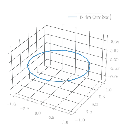
Now let us try a more elaborate example.

Example

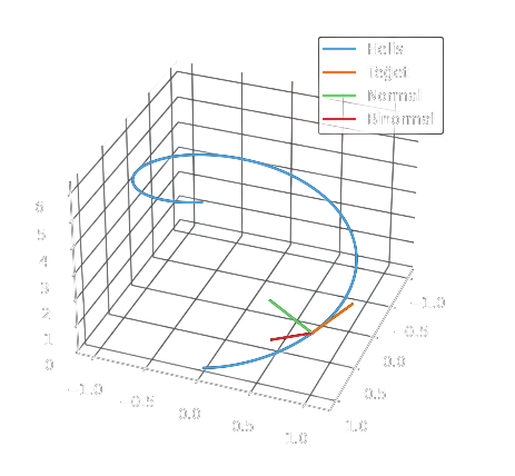
In this example, we will find the Frenet frame of the curve $\alpha : [0, 2\pi) \to E^{3},\ \alpha(t)=(\cos t,\sin t,t)$. This curve is called a helix. Note that in this example $t$ is not our arc-length parameter. That is no problem, however, because we can write the Python code accordingly.

import sympy as smp
from sympy import *
import numpy as np
import matplotlib.pyplot as plt
from sympy.plotting import plot_parametric
#Kütüphaneleri indirdik.
x=smp.symbols("x",real=True,pos=True)#Değişkenimizi(yay uzunluğu parametremiz) ta
r=smp.Matrix([smp.cos(x), smp.sin(x), x])#Eğrimizi tanımlıyoruz.
v=smp.diff(r,x)#Eğrinin teğetini tanımlıyoruz.
T=v/v.norm()#Birim Teğeti tanımlıyoruz.
kappa=smp.diff(T,x).norm()/v.norm()#Eğriliği hesaplatıyoruz.
N=smp.diff(T,x)/smp.diff(T,x).norm()#Normali hesaplatıyoruz.
B=T.cross(N)#Binormali hesaplatıyoruz
tau=smp.diff(B,x).norm()/v.norm()#Burulmayı hesaplatıyoruz.
# Binormal
binormal_Line=r+t*B
# Normal
normal_Line=r+t*N
# Teğet
tangent_Line=r+t*T
ax = plt.figure().add_subplot(projection='3d')#Eğriyi çizdiriyoruz.
xx = np.linspace(0, 2*np.pi, 100)
rr_1 = smp.lambdify([x],r[0])(xx)
rr_2 = smp.lambdify([x],r[1])(xx)
rr_3 = smp.lambdify([x],r[2])(xx)
# Binormal Line 
bb_1 = smp.lambdify([x, t],binormal_Line[0])(1, xx/10) bb_2 = 
    smp.lambdify([x, t],binormal_Line[1])(1, xx/10) bb_3 = smp.lambdify([x, t],binormal_Line[2])(1, xx/10)
 # Normal Line
  nn_1 = smp.lambdify([x, t],normal_Line[0])(1, xx/10) nn_2 = 
    smp.lambdify([x, t],normal_Line[1])(1, xx/10) nn_3 = smp.lambdify([x, t],normal_Line[2])(1, xx/10)
 # Tangent Line
  tt_1 = smp.lambdify([x, t],tangent_Line[0])(1, xx/10) tt_2 = 
    smp.lambdify([x, t],tangent_Line[1])(1, xx/10) tt_3 = smp.lambdify([x, t],tangent_Line[2])(1, xx/10) ax.plot(rr_1,rr_2,rr_3, label='Helis') 
ax.plot(tt_1,tt_2,tt_3, label='Teğet') 
ax.plot(nn_1,nn_2,nn_3, label='Normal') 
ax.plot(bb_1,bb_2,bb_3, label='Binormal') 
ax.legend() 
plt.show()

Running this code displays the helix and the tangent, normal, and binormal vectors at the point corresponding to $t=1$.

In the Next Chapter...

In this chapter, we defined the Frenet frame of a curve and worked through several examples. In the next, we will see how the Frenet frame reveals the characteristic properties of a curve—for example, what happens when its curvature is positive, or when its torsion is zero. We will look at torsion geometrically, and so on. Take very good care of yourselves!