The Concept of a Curve

Curves in Three-Dimensional Euclidean Space

Definition

A curve in $E^3$ is a rule of the form $\alpha : I \subset \mathbb{R} \to E^3$. If $\alpha$ is differentiable (by differentiability here, we mean that its coordinate components are differentiable), it is called a differentiable curve. [1]

⚠️ From this point onward, whenever we speak of a curve, we will assume that it is differentiable unless stated otherwise.

Definition

Let $\alpha : I \subset \mathbb{R} \to E^3$ be a curve. If, for every $t \in I$,

$$\alpha'(t) \neq 0$$

then the curve is called a regular curve.

⚠️ Unless stated otherwise, every curve discussed in this series will be assumed to be regular.

There is something we should question here. Why do we call a curve “regular” when its derivative is nowhere the zero vector? What happens if its derivative is the zero vector at some point? Be patient for just a moment; you will soon see why.

Definition

Consider the curves $\alpha^{*} : I^{*} \subset \mathbb{R} \to E^{3}$ and $\alpha : I \subset \mathbb{R} \to E^{3}$. If there exists a diffeomorphism $\phi : I^{*} \to I$ such that

$$\alpha^{*}(t) = (\alpha \circ \phi)(t)$$

then $\alpha^{*}$ is called a reparametrization of $\alpha$ (in plainer terms, another parametrization of it). [2]

⚠️ A diffeomorphism is an invertible function (that is, a bijection) such that both the function itself and its inverse are differentiable.

Definition

Let $\alpha : I \subset \mathbb{R} \to E^{3}$ be a curve. Its arc length over an interval $[t_0, t]$ is calculated by

$$s(t) = \int_{t_0}^{t} \|\alpha'(\xi)\|\, d\xi$$

If $\|\alpha'(t)\| = 1$ for every $t \in I$, the curve is said to be parametrized by arc length, and the parameter $s$ is used in place of $t$ to indicate this. In other words, when we see the notation $\alpha(s)$, we understand that the curve $\alpha$ is parametrized by arc length. [1]

You should now understand why such a curve is called regular. If $\alpha'(t^{*}) = 0$ for some $t^{*} \in I$, then

$$\left.\frac{ds}{dt}\right|_{t=t^{*}} = \|\alpha'(t^{*})\| = 0$$

This may appear harmless, but something conflicts with the notion of length. The length function must increase continuously because every point you add to the curve increases its length; according to this equation, however, that does not happen. The situation thus contradicts our understanding of length, and this is why regular curves are called “regular.”

Example

Let the curve $\alpha : [0,1] \to E^{3}$ be defined by $\alpha(t) = (t, t^{2}, t-1)$. Since $\alpha'(t) = (1, 2t, 1) \neq 0$, $\alpha$ is a regular curve.

Example

Let the curve $\alpha : [0,1] \to E^{3}$ be defined by $\alpha(t) = (t^{2}, t^{3})$. This curve is called a semicubical parabola. Since $\alpha'(t) = (2t, 3t^{2})$, we have $\alpha'(0) = 0$; the curve is therefore not regular.

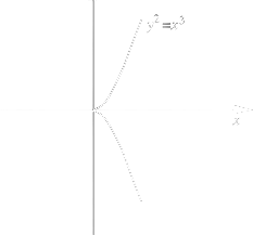
From the graph in the semicubical-parabola example [3], we see that $\alpha(0)$ has a cusp at $t = 0$, the point where regularity fails. This is no coincidence: at the points where nonregular curves fail to be regular, they have cusps.

Theorem

Every reparametrization of a regular curve is regular. [2]

Proof.

Let $\alpha : I \subset \mathbb{R} \to E^{3}$ be a regular curve and let $\alpha^{*} : I^{*} \subset \mathbb{R} \to E^{3}$ be a reparametrization of it. Thus, there exists a diffeomorphism $\phi : I^{*} \to I$ such that

$$\alpha^{*}(t) = (\alpha \circ \phi)(t)$$

It follows that

$$\frac{d\alpha^{*}}{dt}=\frac{d(\alpha\circ\phi)}{dt}=\frac{d\alpha}{d\phi}\frac{d\phi}{dt}$$

Because $\phi$ is a diffeomorphism, its derivative cannot vanish anywhere; if it did, we could not speak of the inverse of $\phi$. The derivative of $\alpha$ must be different from the zero vector because $\alpha$ is regular. Hence the right-hand side cannot be zero, and therefore neither can the left-hand side. Thus $\alpha^{*}$ is regular. □

Example

Let the curve $\alpha : \mathbb{R} \to E^{3}$ be defined by $\alpha(t) = (t, t^{2}, 0)$. This curve is a parabola in the $xy$-plane. We can also describe the same curve as $\beta : \mathbb{R} \to E^{3}$ defined by $\beta(t) = (t^{3}, t^{6}, 0)$; after all, their graphs show the same curve. But at $t = 0$, $\alpha$ is regular while $\beta$ is not. How can a curve be both regular and nonregular? It cannot, of course, because $\beta$ and $\alpha$ are related by

$$\beta(t) = \alpha(t^{3})$$

The function $\phi(t) = t^{3}$ is not a diffeomorphism, so $\beta$ is not a reparametrization.

Example

Let the curve $\alpha : [0, 2\pi) \to E^{3}$ be defined by $\alpha(t) = (\cos t, \sin t, 0)$. This is nothing other than the unit circle in the $xy$-plane. Let us calculate the arc length of this circle.

$$s(t) = \int_{0}^{t} \|\alpha'(\xi)\|\, d\xi$$

Here, $\alpha'(t) = (-\sin t, \cos t, 0)$, so $\alpha$ is a regular curve (the sine and cosine functions are never simultaneously zero). Moreover, $\|\alpha'(\xi)\|=\sqrt{\sin^{2}\xi+\cos^{2}\xi}=1$. Thus our arc-length function $s(t)$ is

$$s(t)=\int_{0}^{t} dt = t$$

We can make several observations about this. First, if we want the entire arc length of the curve, we should look at $t=2\pi$, which confirms the formula for the circumference of a circle (you know, that “two pi r” thing taught in high school). Second—and far more importantly—we see that $t$ is the same as the arc-length parameter, meaning our circle is parametrized by arc length. From calculus, we know that the derivative of a vector-valued function is tangent to that vector-valued function. The tangent to our circle $\alpha$ is therefore the curve $\alpha'$. As the graphs below show, $\alpha$ and $\alpha'$ also have the same image.

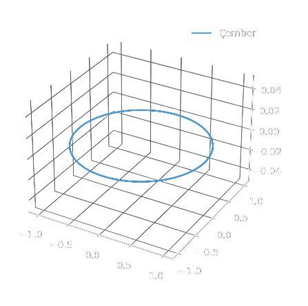
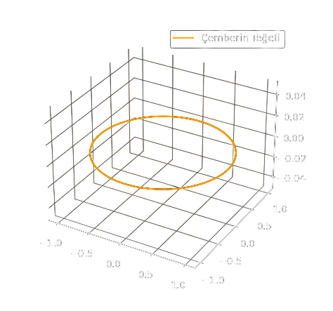
In other words, the derivative of the circle is itself a reparametrization of the circle (you can go ahead and exhibit the diffeomorphism). Are we finished? Not yet. Although they trace the same graph, they do not do so along the same path. The reason is a simple fact of geometry: the radius of a circle is perpendicular to its tangent. Why is that? Ah yes, kings of the cram-school classroom, geometry teachers named Burak—you laughed... you laughed... Let us explain.

$$\langle \alpha(s), \alpha(s)\rangle = \|\alpha(s)\|^{2} = \cos^{2}s + \sin^{2}s = 1$$

If we differentiate the far-left and far-right sides of these equalities with respect to the parameter $s$ (I will never forget my differential geometry professor saying that if you know nothing else, differentiate everything you see in this course—something is bound to come out of it...)

$$\frac{d}{ds}\langle \alpha(s), \alpha(s)\rangle = \langle \alpha'(s), \alpha(s)\rangle + \langle \alpha(s), \alpha'(s)\rangle = 2\langle \alpha'(s), \alpha(s)\rangle = 0$$

we obtain the expression above. Therefore $\langle \alpha'(s), \alpha(s)\rangle = 0$, which means $\alpha' \perp \alpha$. So we have arrived at what our geometry teacher told us years ago, plastic cup in hand: “The radius is perpendicular to the tangent!” Teachers, you have our respect...

Joking aside, this actually gives us an idea: parametrizing a curve by arc length gives us, after just one differentiation, another curve perpendicular to it. We will call this curve the tangent.

Definition

The unit tangent curve of $\alpha : I \to E^{3}$ is denoted by $T(s)$ and defined by $T(s) = \alpha'(s)$.

Theorem

Let $T(s)$ be the unit tangent of the curve $\alpha : I \to E^{3}$. Then $T(s) \perp \alpha(s)$ for every $s \in I$.

Proof.

Because $\alpha(s)$ has an arc-length parametrization, $\langle \alpha(s), \alpha(s)\rangle = 1$. Differentiating both sides with respect to $s$, we obtain

$$\frac{d}{ds}\langle \alpha(s), \alpha(s)\rangle = \langle \alpha'(s), \alpha(s)\rangle + \langle \alpha(s), \alpha'(s)\rangle = 2\langle \alpha'(s), \alpha(s)\rangle = 0$$

It should not be difficult to conclude from this that $\alpha' \perp \alpha$. □

Everything is lovely in theory: if we have a curve parametrized by arc length, we can find its tangent very easily. (We will simply say “tangent” rather than “unit tangent”; non-unit tangents are of no consequence to us!) But you and I both know that life is not always a bed of roses. What can we do if the curve before us is not given in terms of the arc-length parameter? We have two options.

1. We can try to calculate the arc-length parameter: solve the given integral for $s$ and attempt to express the parameter $t$ in terms of $s$.

2. Although the first option is always possible in theory, it is not always practical. In that case, we can use the chain rule:

$$\frac{d\alpha}{dt} = \frac{d\alpha}{ds}\frac{ds}{dt} = \frac{d\alpha}{ds}\|\alpha'(t)\|$$

Since $T(s)=\frac{d\alpha}{ds}$,

$$\frac{d\alpha}{dt} = T(s(t))\|\alpha'(t)\|$$

and hence

$$T(t)=\frac{1}{\|\alpha'(t)\|}\frac{d\alpha}{dt}$$

If you noticed that I gradually shifted the parameter of $T$ from $s$ to $t$, I can do this because $s$ is itself a function of $t$. We have consequently found a way to calculate the tangent curve without ever converting to the arc-length parameter. Let us now apply it.

Example

Let the curve $\alpha : [0, 2\pi) \to E^{3}$ be defined by $\alpha(t) = (4\cos t, \sin t, t)\alpha(t) = (2\cos t, \sin t, t)$. This curve is called an elliptical helix. We will calculate its tangent using the formula obtained above. We will not do it by hand, however; we will use Python, employing the SymPy library to carry out the calculation easily. We will then plot the curves using NumPy and matplotlib. The calculation is performed with the following script.

import sympy as smp
from sympy import *
import numpy as np
import matplotlib.pyplot as plt
# parametrenin oluşturulması
t=smp.symbols('t')
# eğrinin oluşturulması
alpha=smp.Matrix([4*smp.cos(t),smp.sin(t),t])
# eğrinin türevi
alpha_turev=smp.diff(alpha)
# T vektörünün oluşturulması
T=alpha_turev/alpha_turev.norm()
# Çizdirilecek aralığın oluşturulması
tt=np.linspace(0,2*np.pi,100)
# x, y, z eksenlerinin oluşturulması
ax = plt.figure().add_subplot(projection='3d')
# eğrinin ve teğetinin koordinat bileşenlerinin NumPy kütüphanesine aktarılması
rr_1=smp.lambdify([t],alpha[0])(tt)
rr_2=smp.lambdify([t],alpha[1])(tt)
rr_3=smp.lambdify([t],alpha[2])(tt)
rrp_1=smp.lambdify([t],T[0])(tt)
rrp_2=smp.lambdify([t],T[1])(tt)
rrp_3=smp.lambdify([t],T[2])(tt)
# Grafiğin oluşturulması
ax.plot(rrp_1,rrp_2,rrp_3, label='Teğet',color='orange')
ax.plot(rr_1,rr_2,rr_3,label='Eğri')
ax.legend()
plt.show()

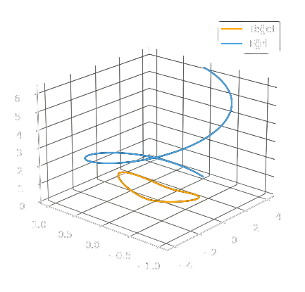
As you can see, the tangent vector rather resembles a Pringles chip. Readers without programming experience should, of course, take out pencil and paper and solve it themselves. Still, I will write the result here in case you would like to check your work:

$$T(t)=\left( -\frac{4\sin(t)}{\sqrt{15\sin^{2}(t)+2}}, \ \frac{\cos(t)}{\sqrt{15\sin^{2}(t)+2}}, \ \frac{1}{\sqrt{15\sin^{2}(t)+2}} \right)$$

Conclusion and the Next Chapter...

In this chapter, we discussed the concept of a curve and some of its properties. In the next chapter, we will add new definitions to curves and make them more meaningful. Later chapters will turn to several special curves. Take care!

References

[1] Do Carmo, M. P. (2016). Differential geometry of curves and surfaces: revised and updated second edition. Courier Dover Publications.

[2] Pressley, A. N. (2010). Elementary differential geometry. Springer Science & Business Media.

[3] Visualizing Differentials in Two and Three Dimensions - Scientific Figure on ResearchGate. Available from: https://www.researchgate.net/figure/a-semi-cubical-parabola_fig4_37143313 [accessed 8 Apr, 2022]